Local fields and a traveling wave
The static electromagnetic-wave figure remains available below. Interactive controls require JavaScript and a web server rather than file://.
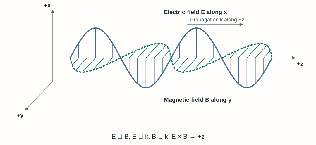
Explore: local fields and a traveling wave
Watch one fixed observation position while the wave pattern travels past it.
The arrow tails stay at (0, 0, z₀). Their signed lengths oscillate: E points along x and B along y. The faint arrows sample other fixed positions; they are field values, not moving particles.
Time is greatly slowed: 1× displays one optical period in 4 seconds. Playback speed changes the display rate, not the physical wave speed.
The spatial pattern travels toward +z
E · solidB · dashed● fixed observation position
At the selected position
Transverse view, looking along +z (into the page).
- Time, t/T
- 0.000
- Signed Eₓ/E₀
- 1.00
- Signed Bᵧ/B₀
- 1.00
Paused. Click Play to start, or Step to advance by 1/32 of an optical period.
Model: source-free traveling plane wave in a homogeneous, lossless medium. Eₓ/E₀ = Bᵧ/B₀ = cos[2π(z/λ − t/T)], with constant phase offset φ₀ = 0. E and B oscillate in phase. Separate normalized field scales and schematic perspective are used; equal arrow lengths do not mean equal physical units. Physically, B₀ = E₀/v.
The phase pattern and electromagnetic energy propagate toward +z at v = λ/T. At each fixed position, the local fields change with time. Moving the position control chooses a different observation position; it does not move a field object.