Build a pattern from spatial frequencies
Open through a web server with JavaScript enabled to use this interactive explorer. Figure 2.9 remains the static reference.
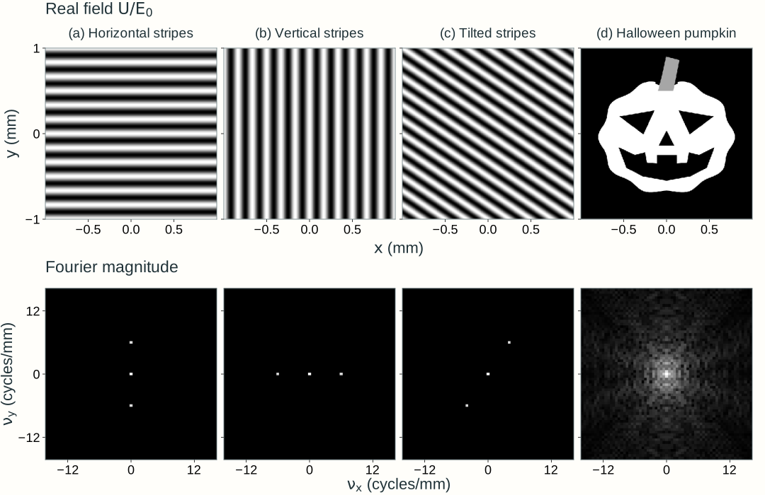
Explore: build a pattern from spatial frequencies
Choose an input, inspect a frequency pair, and change which frequencies contribute to reconstruction.
Grayscale specifies a real electric-field amplitude with uniform phase. These panels show fields, not optical intensity. The output is a Fourier reconstruction.
Input field
Fourier magnitude
Selected frequency pair
Reconstructed field
Black is zero; white is 1. Orange marks negative field; blue marks values above 1. The scale stays fixed.
Its display is normalized for visibility; the actual contribution amplitude is reported above.
Low pass includes frequencies inside and on the solid circle; high pass includes frequencies outside it. The crosshair inspects a component; the dashed marker identifies its opposite-frequency partner. Inspection does not change the filter. Only the central spectrum, ±16 cycles/mm, is displayed. Pass all includes frequencies beyond this view.
Model, numerical method, and validation
The input is a real nonnegative field U/E₀ with uniform phase on a 2 × 2 mm window, sampled on a 256 × 256 grid. Stripes repeat across this window. The pumpkin and letter F have a zero border, but the discrete Fourier calculation still uses periodic boundary conditions. A sharp circular cutoff can cause ringing, including negative reconstructed field values; they are retained rather than clipped from the calculation.
A negative-exponential two-dimensional FFT supplies complex coefficients c, normalized by the sample count. The physical field spectrum is the window area times E₀c. Low pass retains a coefficient when √(νₓ² + νᵧ²) ≤ νc, including equality; high pass retains its complement, √(νₓ² + νᵧ²) > νc. Both retain the transmitted coefficients’ phases. The inverse FFT reconstructs the field. At zero cutoff, low pass retains only DC, while high pass removes only DC. Pass all bypasses either filter and reconstructs the original sampled input.
For a real input, c(−νₓ,−νᵧ) is the complex conjugate of c(νₓ,νᵧ). The lower panel displays their real combined contribution 2|c| cos[2π(νₓx + νᵧy) + arg(c)], normalized to unit peak for visibility. The zero-frequency component is a constant and is counted once. A negligible coefficient has no appreciable contribution; its phase is not interpreted.
The spectrum displays log(1 + 100m)/log(101), where m is magnitude divided by the largest magnitude for that input. The cutoff and selection never renormalize this spectrum. The shared input/output color scale is fixed from −0.5 to 1.5; any values outside that display range are explicitly reported. A normalized coefficient amplitude and phase accompany the selected pattern. Analytical stripe coefficients, complementary low/high-pass reconstructions, FFT round trips, DC and all-pass limits, conjugate symmetry, Parseval, and an independent NumPy reference validate the calculation.