Filtering a coherent field
Open through a web server with JavaScript enabled to use this interactive explorer. The static 4-f relay reference is shown below.
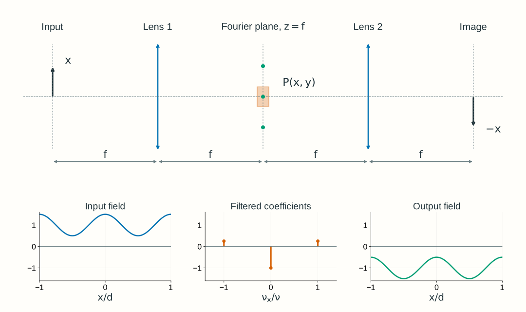
Explore: filtering a coherent field
Select a preset, then change the spatial frequency, mask width, or central component's phase. Predict the output before inspecting its intensity.
Coherent periodic field, uniform in y, in air: λ = 600 nm and f₁ = f₂ = 100 mm. The ideal 4-f relay has unit magnitude of magnification and inversion. The input is at z = −f, the mask at z = +f, and the output at z = 3f; the lenses are at z = 0 and z = 2f. Only the Fourier-plane mask limits transmission. Each plane uses the same transverse coordinate names x,y; these do not imply direct input-position-to-output-position mapping.
- Side-order positions at z = +f
- Orders transmitted
- Mean output / input intensity
Input at z = −f: a constant plus two tilted components
Uin(x,y) = U(x,y,−f), with Uin/E₀ = 1 + 0.5 cos(2πνx). The input is real and positive; the plotted curve is its field amplitude, not intensity.
Fourier plane at z = +f: select amplitude and phase
Dashed stems: incident coefficients. Solid stems: transmitted magnitudes; labels give the applied phase. The shaded opening is −a ≤ x ≤ a. The ideal periodic field has three discrete spectral lines; their drawn widths are not physical spot widths.
Output at z = 3f: reconstruct the field, then square
Uout(x,y) = U(x,y,3f). Field curves show V = Uout/(G E₀), with the uniform relay phase G removed for display: solid Re(V), dashed Im(V). Intensity is |V|² = Iout/I₀, where I₀ = ½ϵ₀cE₀². All plot scales remain fixed.
Model, numerical method, and validation
The normalized input is 1 + m cos(2πνx), with m = 0.5. Its coefficients at −ν, 0, +ν are m/2, 1, m/2. Spatial frequencies ν are in cycles/mm; their positions in the Fourier plane z = +f are xⱼ = λfνⱼ. A position x there selects input spatial frequency ν = x/(λf); position and spatial frequency remain different physical quantities. The ideal slit passes an order when |xⱼ| ≤ a, including equality. A phase shift ψ₀ acts only on the central order. This is a discrete periodic one-dimensional teaching model, uniform in y, with large ideal lens apertures except for the Fourier-plane mask. It does not calculate a finite illuminated pupil, physical spot widths, or a microscope PSF.
The equal-f 4-f relay reconstructs Uout(x)/E₀ = G Σ cⱼPⱼ exp(−i2πνⱼx), with G = −exp(i4kf), k = 2π/λ. Returned fields retain G; only the displayed real and imaginary curves divide it out. The minus sign on x accounts for inversion. The symmetric input hides inversion visually; the model is also tested with an asymmetric complex input.
The browser evaluates these three components directly, without an FFT. Curves use 401 samples on x = ±0.2 mm, giving at least 50 samples per period over the selected frequency range. The plotted intensity scale is fixed at 0–4 relative to I₀; each curve is not separately normalized. The mean intensity over one period equals the sum of squared coefficient magnitudes. Thus a phase-only mask preserves mean intensity while blocking side orders reduces it. Because this periodic field extends indefinitely, this mean is a per-period comparison, not a finite total beam power.
Analytical coefficient, inversion, phase, and Parseval tests plus an independent NumPy FFT reconstruction validate the selected presets and control limits. Doubling the plot sampling checks the maxima and period-averaged intensities. These teaching calculations do not set Lab 2 software requirements.