Lens phase and field propagation
Open through a web server with JavaScript enabled to use the interactive explorer. The static lens-phase reference remains available below.
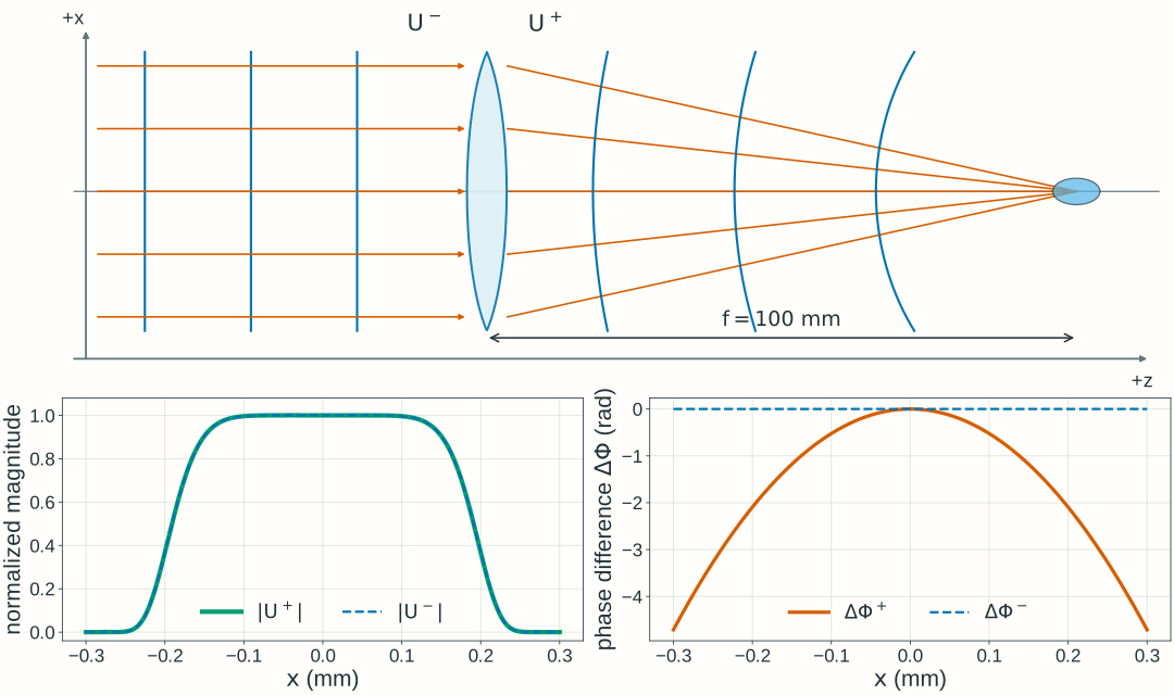
Explore: lens phase and field propagation
Predict the phase immediately after a lens, then choose a downstream plane and inspect the propagated field intensity.
Stationary scalar, monochromatic fields in air, λ₀ = 600 nm, with the exp(−iωt) convention. An ideal thin lens changes phase at z = 0. Downstream propagation uses the forward, paraxial free-space approximation for the two-dimensional field.
- Output curvature, 1/Rout
- Signed output radius, Rout
- Geometric axis crossing
Relate phase curvature to the ray picture
Fixed z = −200 to +250 mm; x = ±2.5 mm. Dashed geometric wavefronts and solid rays use the same physical coordinate mapping. The axes have different scales, so physical right angles need not appear as 90° on screen; wavefront curvature is almost invisible at this scale. Wavefront spacing is illustrative, not an optical wavelength. This geometric construction does not show the full diffracted field near focus.
At the lens: phase changes, magnitude does not
Before lens · dashedImmediately after · solid
Unwrapped phase difference from the on-axis value: Φ(x,y;R) − Φ(0,0;R) = kr²/(2R). The lens adds −kr²/(2f) to this difference. The amplitude A(r) and local intensity are unchanged at the lens plane; axes stay fixed at x = ±1 mm and phase difference = ±90 rad.
After propagation: a different intensity distribution
Input intensity · dashedObserved intensity · solid
This is the y = 0 central cut of a two-dimensional calculation, not a one-dimensional propagation model. Fixed central view x = ±0.3 mm; fixed intensity scale 0–2500, normalized to the input peak. The broader input and defocused profiles extend outside this central view. The input peak is 1 on this scale; focusing makes the observed peak much larger. A finite illuminated field gives finite intensity near the geometric axis crossing. The plotted intensity is cycle averaged; L selects a plane, not a time.
Model, numerical method, and validation
The dimensionless input magnitude is A(r)/E₀ = exp[−(r/w)⁸], with w = 0.8 mm. This is a smooth circular illumination profile; w is its scale radius, not a Gaussian-beam waist. Its scale diameter is 1.6 mm; the smooth profile has no hard edge. This larger illuminated region places the wave-intensity maximum close to the geometric axis crossing, although finite-aperture diffraction can shift it slightly. The input on-axis phase and the lens’s uniform phase delay are chosen as zero reference values. The lens multiplies the field by exp[−ikr²/(2f)]. The finite field continues to spread even when its phase immediately after the lens is planar.
The input peak electric-field amplitude E₀ is measured in V/m. The numerical field uses U/E₀, and intensity is normalized to the same input peak across settings, rather than to each curve’s own peak. The meridional picture shows geometric rays and wavefronts in physical coordinates with unequal axis scales; it is not a calculation of the full diffracted field or intensity along a ray.
Propagation uses a 1024 × 1024 square field on x,y ∈ [−3, 3) mm (5.859375 µm spacing). The paraxial transfer factor is exp(ikL) exp[−iL(kₓ² + kᵧ²)/(2k)]. Returned complex samples represent the full U/E₀, including the common axial phase exp(ikL); that common phase does not change intensity. For plotting, the complex central field is Fourier-interpolated to 1.464844 µm spacing before taking its squared magnitude; this does not add physical resolution to the two-dimensional simulation. The full two-dimensional power integral is conserved by this phase-only propagation in a common medium.
Checks compare zero-distance identity, curvature signs, integrated power, and central profiles after grid and window refinement. At the selected boundary/reference cases, doubling the sample count changes the central complex field and intensity by less than 10⁻⁸ of input peak field and intensity, respectively; doubling the window at fixed spacing changes them by less than 10⁻⁶ and 10⁻⁶, respectively. Independent radial Fresnel integrals also check the narrow focal profiles and axial peak positions. The finite FFT window is periodic; these checks apply to the stated controls, illumination, and viewing region.
The reference calculations use NumPy/SciPy; the browser evaluates the same scalar model in JavaScript. Check spatial sampling, numerical window, and refinement before interpreting a computed peak. These numerical teaching choices do not set Lab 2 software requirements.