Change the pupil and inspect image quality
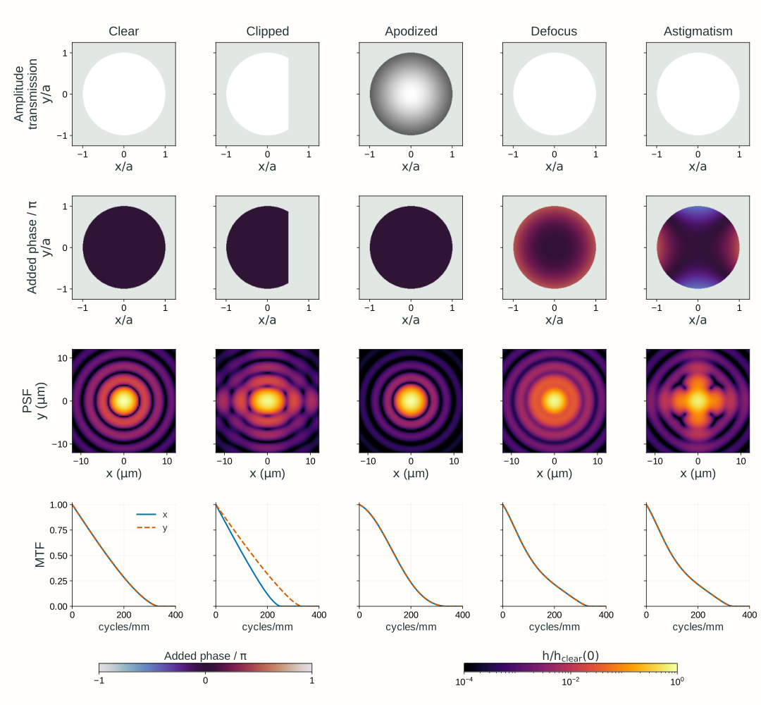
Open through a web server with JavaScript enabled to use the interactive explorer. Figure 2.17 provides a static comparison.
Explore: change the pupil and inspect image quality
Compare pupil transmission, the intensity point response, and retained sinusoidal contrast.
An on-axis point at infinity supplies a uniform plane wave to an ideal lens at z = 0. A complex pupil immediately after the lens changes amplitude transmission and adds phase; the sensor stays at z = f. This scalar paraxial model is in air, with image-space NA ≈ a/f. The phase panel shows the additional pupil phase, ψ, with the ideal lens phase accounted for separately.
Power vs clear pupil at the same NA100.0%
Clear-pupil first-dark-ring radius3.66 μm
Clear-pupil incoherent cutoff333 cycles/mm
Pupil amplitude transmission
Amplitude: 0 → 1
Additional pupil phase, ψ
Phase: −π → +π
Intensity PSF, h
Fixed log scale: 0 → 0.36 μm⁻²
PSF profiles through the axis
Directional incoherent MTF
x direction y direction clear-pupil reference at the selected λ₀ and NA
The PSF has unit integral over the full numerical plane; it is not renormalized to the cropped picture or to its peak. Brightness scales stay fixed as controls change. Power is reported relative to a clear pupil at the same selected NA; it does not compare absolute collected power between different NA settings. The first-dark-ring radius and cutoff above describe the clear reference pupil; altered pupils need not have the same spot shape or usable contrast.
Model, numerical method, and validation
The uniform incident amplitude is unchanged between pupil presets. The pupil amplitude panel shows transmission tₚ; the transmitted amplitude is the incident amplitude multiplied by tₚ. Changing NA changes the ratio a/f, rather than moving the object to a finite distance. With added defocus, the best focus can move, but the sensor remains at the reference plane z = f.
The reference pupil uses dimensionless coordinates x/a,y/a, with ρ² = (x/a)² + (y/a)² ≤ 1. Clear transmission is one. Clipping removes the cap x/a > 0.5. Apodization uses amplitude transmission exp(−ρ²), rather than intensity transmission. Defocus adds phase ψ = 2πwρ²; astigmatism adds 2πw[(x/a)² − (y/a)²]. The coefficient w is in waves; it is not an RMS wavefront error. Phase-only presets preserve transmitted power. The symmetric astigmatism case can have coincident x and y MTF profiles at this observation plane.
The calculation samples tₚ exp(iψ) across a 128-sample pupil diameter and zero-pads it to a 512 × 512 array. This pupil factor follows after accounting for the ideal lens phase and propagation to z = f. A centered negative-exponential FFT supplies the amplitude response up to phase factors and a uniform magnitude scale that do not affect the normalized intensity PSF. Its squared magnitude is normalized by the full numerical-plane intensity integral to obtain h in μm⁻². The physical PSF spacing is λ₀/[NA N Δ(x/a)], with wavelength in micrometers. Changing wavelength or NA changes that spacing; the rendered viewing axes remain fixed. Profiles and the image use interpolation between computed samples.
The MTF describes imaging of mutually incoherent object points near the axis: their image intensities add, while contributions across the pupil for each individual point add as fields. It is not the transfer function for the coherent intensity of an extended plane-wave pattern. The Fourier transform of h gives the complex incoherent OTF. Its magnitude is the MTF; normalization gives MTF(0) = 1. Padding is large enough to contain the linear pupil autocorrelation, avoiding circular overlap. Clear-pupil references use the analytical Airy response and circular-pupil MTF. Finite pupil sampling produces small edge-discretization errors; refinement checks test them. Full-plane normalization, phase-only power conservation, directional anisotropy, and analytical Airy/MTF comparisons validate this numerical model.
The PSF map uses a fixed logarithmic brightness transform log(1 + 100 h/0.36)/log(101), with h in μm⁻². Both profile plots use fixed axes. The model is a scalar, monochromatic, paraxial, locally shift-invariant point response; high-NA vector effects, broadband light, camera pixels, and a full real-lens prescription are outside this explorer. No student software installation is required.