Real lenses and image quality

The engineering question

Our system forms an image and its bundles clear the apertures. Does it preserve enough detail and contrast to distinguish the features we care about? The coverage checks in Chapter 1.5 are necessary, but real curved surfaces can spread even a well-focused point. We now connect that spreading to a task: retaining contrast at a specified feature spacing.

A lens element is a sequence of surfaces

An ideal thin lens changes ray angle at one plane. A real singlet has two refracting surfaces separated by glass. At each surface the ray changes direction according to the local normal:

The angles here are measured from the surface normal, not the optical axis. Because a curved surface has different normals at different heights, high rays need not meet at the paraxial image. The refractive index also depends on wavelength, n(\lambda); this dispersion can give different colors different focal positions.

To move from an ideal thin lens to a real-lens model, we describe its geometry and materials in an optical prescription. Sequential ray-tracing tools such as Optiland use this surface-by-surface description, illustrated by the singlet table below. Read a prescription one surface at a time. A positive curvature radius places the center of curvature toward positive z from the surface vertex; a negative radius places it toward negative z. The vertex is the point where the surface intersects the optical axis. Thickness means the distance to the next vertex, and the material listed after a surface fills that next interval. Clear semi-diameter means the radius of the usable opening. Neither a curvature radius nor a clear aperture is a focal length.

This illustrative singlet has a 3 mm-radius iris immediately before its front surface; both refracting surfaces have 3.5 mm clear radii. The refractive index is specified only at 550 nm: this is an artificial monochromatic teaching prescription, not a catalog glass or a dispersion model.

For the object at z_\mathrm{o}=-90~\mathrm{mm}, paraxial ray-transfer-matrix (RTM) analysis of this prescription gives image coordinate z_\mathrm{i}\approx48.8315~\mathrm{mm} and magnification M\approx-0.5056. The distance from the rear vertex to that image is therefore 48.8315-4=44.8315~\mathrm{mm}. This is the paraxial reference plane; finite-aperture real rays need not have their smallest blur there. The effective focal length (EFL) describes the lens's paraxial focusing power; with air on both sides, it is calculated as f_\mathrm{eff}=-1/C\approx30.6818~\mathrm{mm}, where C is the lower-left entry of the lens's ray transfer matrix for the (x,\theta) ray state.

Principal planes give the paraxial distance references

Commercial lens specifications often list effective focal length f_\mathrm{eff} and back focal distance (BFD). For an object at infinity, both describe the paraxial focus, but from different references: EFL is measured from the image-side principal plane, while BFD is measured from the rear surface vertex. Surface-vertex coordinates are sufficient for ray tracing, but to reuse the familiar lens equation at a finite object distance, we need the principal-plane references. Treating EFL as a distance from a lens surface can place the sensor incorrectly.

A thick lens has an object-side principal plane H_1 and an image-side principal plane H_2. These are mathematical planes for first-order imaging, not refracting surfaces, aperture stops, or necessarily the center of the glass. They need not even lie inside the lens. For this singlet at 550 nm, the front and rear surface vertices are at z=0 and z=4~\mathrm{mm}, while z_{H_1}=1.3636~\mathrm{mm} and z_{H_2}=2.6364~\mathrm{mm}.

Keep all positions on the chapter's global z axis, positive along propagation. For paraxial imaging with the same exterior medium on both sides, define signed offsets from the appropriate principal planes, then use the familiar signed relation:

The offsets are signed, not positive distances: for a real object to the left and a real image to the right, \ell_\mathrm{o}<0 and \ell_\mathrm{i}>0. Convert the result back to a sensor coordinate with z_\mathrm{i}=z_{H_2}+\ell_\mathrm{i}. The focal point F_2 is the image of an object at infinity: here it is at z_{F_2}=z_{H_2}+f_\mathrm{eff}=33.3182~\mathrm{mm}, so its distance from the rear vertex is 33.3182-4=29.3182~\mathrm{mm}. At another wavelength, dispersion may change both focal length and principal-plane locations; the physical object, lens, and sensor coordinates stay fixed during a spectral comparison.

Before trusting a spot plot, specify the object conjugate, field point, wavelength, stop, clear apertures, and image plane. Changing any of these changes the question being answered.

Recognize what refocusing can—and cannot—fix

Defocus means the sensor is away from a chosen best image plane. Moving it can shrink a spot, but cannot generally bring all real rays and wavelengths to one point. The following signatures help choose a useful next design change.

These effects can occur together. An achromat reduces selected chromatic errors; it does not make every field and wavelength perfect. Likewise, stopping down can reduce geometric aberration but also changes throughput and diffraction. Judge the complete requirement rather than a single attractive spot.

Read spots and ray fans as complementary diagnostics

A spot diagram plots where sampled rays meet an image plane. A ray fan shows how the image-position error varies as we select rays along a line across the entrance pupil. The spot shows the resulting shape; the fan shows which pupil zones produce it. Keep the field, wavelength, image plane, reference, and scales the same when comparing designs.

A centroid-referenced RMS spot radius summarizes a weighted second moment:

Here \mathbf r_j is a ray intercept and w_j its weight. A chief-ray reference instead measures displacements from the chief-ray intercept; the two references need not agree. Centering a spot removes its displacement from view, so it cannot by itself establish low distortion.

A straight sloping fan can indicate defocus; curvature that remains after refocusing reveals residual aberration. Inspect more than the on-axis spot: field and wavelength can change both the shape and best focus. Also inspect rejected rays. A smaller spot obtained by clipping troublesome rays may come with unacceptable lost light or field coverage.

From a spot diagram to a point-spread function

The spot diagram tells us where sampled rays land. To understand the resulting image intensity, return to the defocused point in Chapter 1.5. Its rays spread over a disk instead of meeting at one point. A diameter describes the extent of that blur, but not how the light is distributed inside it. The intensity point-spread function (PSF) describes the spatial intensity response to one object point. A uniform blur disk is a useful geometric model under suitable uniform pupil illumination and paraxial conditions; it is not the only possible point response.

A spot diagram is not automatically an intensity PSF. To estimate a geometric intensity distribution, sample the admitted bundle sufficiently and assign the correct light flux to the samples. Count rays in small image regions only when the sampling and weights justify that count as light. A sparse ray sketch conveys paths, not quantitative brightness.

Build an image by adding shifted point responses

Now build an extended object from many points. Each point produces a blur pattern positioned relative to its geometrically mapped image position, scaled by that point’s brightness. Under the local linear intensity-imaging assumption, we add these intensity contributions. If neighboring points have approximately the same PSF shape, their contributions are shifted copies of one pattern. This repeated shift, scale, and addition is convolution. Light spreads from bright regions into neighboring dark regions, softening image detail.

For a general two-dimensional image, this local linear, shift-invariant intensity model gives

Here x,y are transverse image-plane coordinates, u,v are blur offsets, and h(u,v) is the normalized two-dimensional intensity PSF. Its integral over the image plane is one. I_\mathrm{ideal} already includes the geometrical magnification; the convolution describes the additional spreading of that ideal image. Normalizing the PSF separates this spreading from the overall transmitted light level.

The same two-dimensional convolution applies to a stripe pattern that varies along x and remains uniform along y. The PSF can still spread light in both directions and need not be circular or symmetric. The next section uses these stripe patterns to measure how much bright–dark variation survives.

Measure detail with sinusoidal stripe contrast

We can measure how much bright–dark variation survives this mixing with a stripe target. For stripes varying along x and uniform along y, write the sinusoidal intensity as I(x), described by its mean intensity \bar I, modulation m, and spatial frequency \nu:

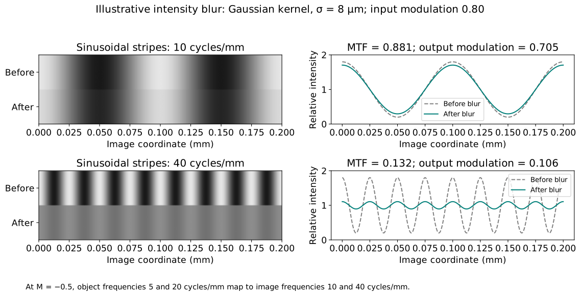
Spatial frequency counts cycles per unit length. One bright–dark cycle is one line pair, so 20 cycles/mm means a 0.05 mm period. Modulation is dimensionless: equal bright and dark intensities give zero; a zero minimum gives one. Use values proportional to the actual light intensity when calculating modulation; processed image pixel values (e.g., gamma-corrected display values) may not preserve that proportionality.

The modulation transfer function (MTF) reports retained sinusoidal contrast versus frequency in a selected direction. For that direction, compare corresponding object and image frequencies:

For M=-0.5, a 20 cycles/mm object pattern becomes a 40 cycles/mm image pattern. Inversion reverses position; it does not make the frequency magnitude negative. Always label whether frequency refers to the object or image, its units, and the direction in which intensity varies. Square-wave bars contain several sinusoidal harmonics, so their measured contrast is not interchangeable with sinusoidal MTF.

MTF is local to a specified field point (an object position). The shift-invariant assumption means nearby points have approximately the same point response within a small field patch; it does not make that response identical across the entire field of view. Off-axis aberrations and clipping can change the retained contrast, so compare separate MTF curves at the center and selected off-axis fields, for each specified frequency direction. Use the local magnification when converting the same object frequency to an image frequency at each field.

Connect the point response to MTF through the Fourier transform

The PSF and MTF describe the same local intensity-imaging behavior in different ways: where a point’s light spreads, and how much sinusoidal contrast survives. Sinusoids are especially useful because a linear shift-invariant system changes their amplitude and phase while retaining their frequency. The optical transfer function (OTF) packages those two changes. The two-dimensional Fourier transform of the intensity PSF h(u,v) gives the OTF as a function of the two image-plane spatial-frequency components \nu_x,\nu_y. Normalize at zero frequency; MTF is the magnitude:

A stripe pattern varying along x and uniform along y has spatial-frequency vector (\nu,0). Its directional MTF is therefore

This selects a direction in the two-dimensional transfer function; it does not replace the PSF with a one-dimensional function. It is the same retained-contrast ratio defined above, evaluated for this stripe direction.

We need linear-systems mathematics for this relationship, not electromagnetic wave theory. OTF phase contains information about shifts or contrast reversals that the nonnegative MTF alone omits. Normalization gives \mathrm{MTF}(0,0)=1 for a nonzero-throughput response; this does not mean all incident light was transmitted.

Fine stripes often lose more contrast because the blur spans a larger fraction of their period. However, the MTF curve need not decrease monotonically; its shape depends on how light is distributed within the PSF.

Choose against a contrast requirement, not just a spot size

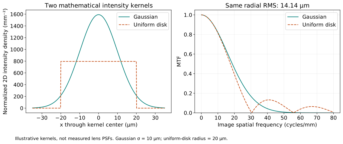
Two distributions can have the same RMS radius but put light in different places. One may be stretched in one direction; another may have a narrow core and broad tails. Their retained contrast can differ at the detail frequency required by the task. A single spot radius cannot encode all of that information.

We now return to the real singlet in Figure 1.19, with its 3 mm-radius front iris and the object at z_\mathrm{o}=-90~\mathrm{mm}. Figure 1.25 compares its on-axis image at 550 nm at the paraxial reference plane and at the refocused plane used in Figure 1.22. The lens prescription and pupil stay fixed; only the sensor position changes. Here the spots and geometric MTF come from the same traced ray distributions, rather than the illustrative kernels in Figure 1.24.

The 0.5 threshold in Figure 1.25 is an illustrative requirement, not a universal pass level. Commercial examples use other values: Edmund Optics compares imaging lenses at 0.30 MTF across the field, gives a metrology example requiring 0.35 at 30 image-space cycles/mm, and illustrates a depth-of-field boundary at 0.20. These are application-specific choices. A threshold is meaningful only with its spatial frequency, field, and operating conditions specified, and with a clear distinction between lens MTF and complete-system MTF.

Define the requirement before optimizing: object detail frequency, required MTF, field, wavelength conditions, and both transverse frequency directions (e.g., tangential, also called meridional, and sagittal). If designs have different magnifications, convert the same object detail to each image frequency. Then evaluate clear apertures, throughput, size, and allowed focus travel alongside contrast. Refocusing is a practical variable; changing a catalog lens’s internal prescription usually is not.

Geometric MTF is an approximation. A properly weighted ray-intercept distribution can estimate the intensity kernel when geometric spreading dominates at the frequencies of interest. It does not contain the diffraction PSF, and is inadequate near diffraction-limited performance. A geometric pass is therefore a pass of the stated ray model, not proof of a physical camera’s measured MTF. Detector pixel integration, sampling, noise, and illumination also affect the complete measurement.

From optical concepts to Optiland

Real lenses can exhibit several aberrations at once, so evaluating image quality means tracing many rays across fields, wavelengths, and sensor positions. Optical simulation software makes these repeated calculations and comparisons practical. Zemax OpticStudio is widely used commercial software for professional optical design. Here we use Optiland, an open-source Python framework for optical design, analysis, and optimization. To get started, follow its guide for optics students and first-time users.

The following examples compare an ideal lens with three commercial lens prescriptions. These are new examples with a 20 mm entrance pupil, distinct from the illustrative 3 mm-radius-iris singlet in Figures 1.19–1.25. Each comparison connects a prescription to rays, spots, focus, and contrast. The calculations use Optiland v0.6.2.

Import the lens, then define the application

When a manufacturer provides a Zemax .zmx prescription, import it rather than retype the surface radii, thicknesses, glass types, and aspheric coefficients. The AL2550-A paraxial excerpt below shows a compact sequence: import the lens, choose the reference wavelength and object position, calculate the paraxial image plane, and put the sensor there. The same workflow applies to other imported lenses. For a full evaluation, also choose the application conditions: aperture stop, pupil diameter, field points, and spectral sampling. Finally, trace rays and evaluate or optimize the stated requirement. A vendor file supplies a lens model; its original object and image settings need not match your application.

The saved figures use a configured comparison model for each lens. The aspheric prescription agrees with the vendor Zemax file, but its application setup has been changed to the conditions below. The spherical prescription was reconstructed from rounded manufacturer catalog geometry, and the achromatic prescription from the manufacturer drawing; their excerpts show these alternatives explicitly. The ideal thin lens is defined directly.

Keep the comparison conditions fixed

For each lens, place the object 150 mm before its front principal plane at 550 nm, with a fixed 20 mm-diameter entrance pupil at the front vertex. Evaluate object heights 0, 5, and 10 mm and wavelengths 486.1, 550, and 656.3 nm. The three spectral lines have equal priority in the pooled RMS calculation. Pupil samples are uniform in area and have equal weights; this teaching model neglects absorption and other transmission losses. Geometry is built once at the 550 nm reference and held fixed while tracing every wavelength; each selected case uses one shared sensor plane for all fields and colors. Global axial coordinates are measured from each lens’s front vertex. Because principal-plane positions and focal properties differ, these common settings do not impose identical NA or exact magnification across the lenses; this is a comparison of specific products under shared conditions.

The paraxial setting uses the 550 nm first-order image prediction. The shared RMS-refocused setting moves only the sensor to minimize the mean squared pooled-color RMS radius across the three fields, with equal field weights. At each field, pool equal numbers of rays from the three wavelengths before calculating one centroid and RMS radius, so color displacement remains part of the blur. RMS is calculated from the spatial spread of these intercepts, not from a Fourier transform. The ideal lens has one setting because its paraxial and best geometric focus coincide.

Read the five panels together

1. a · Ray layout: identify the lens, pupil, object fields, and selected sensor plane.
2. b · Field spots: compare the three object heights at 550 nm on common transverse scales.
3. c · Color spots: compare the on-axis wavelengths at that same sensor plane; they are not independently refocused.
4. d · Focus sweep: locate the selected plane relative to the lens’s own 550 nm paraxial prediction. A shared compromise need not minimize every field or color separately.
5. e · Geometric MTF: compare separate 486.1, 550, and 656.3 nm results on the common 0–20 image cycles/mm grid. At each wavelength, show one on-axis curve, where tangential and sagittal coincide, and outer-field tangential and sagittal curves at 10 mm: nine curves in total. Color identifies wavelength and line style identifies field and direction. Equal image frequency does not represent equal object detail when magnifications differ.

In these Optiland calculations, the meridional coordinate is the software’s y, corresponding to the textbook’s upward transverse coordinate. The orthogonal coordinate is its x; tangential MTF varies along the former and sagittal MTF along the latter. Lengths are in millimeters; wavelength inputs are in micrometers. A field coordinate chooses a scene point, while a pupil coordinate chooses a ray within its bundle.

Optiland traces the rays and supplies the native GeometricMTF analysis used in panel e. Run this analysis separately for each wavelength at the selected shared sensor plane, with scale=False to disable its optional diffraction-limit scaling. These are geometric, monochromatic curves; diffraction, transmission losses, tolerances, and detector effects are excluded. Project analysis code calculates the pooled RMS from equal-weight ray intercepts to select the sensor plane.

Separate wavelength MTF curves diagnose each color’s contrast transfer, but they do not establish the contrast of the combined-color image. Averaging their magnitudes would discard the relative color-image displacement. Panel c compares on-axis color spots on a common reference at the shared sensor plane; off-axis color images can also have different centroids. A combined-color MTF would require combining complex OTFs with a common image-plane reference before taking the magnitude; we do not plot it here.

Native Optiland: evaluate each wavelength at the same sensor plane

# Teaching excerpt showing the key approach; not a standalone script.
from optiland.mtf import GeometricMTF

# optic already has the selected sensor plane and fields with max height 10 mm.
# pupil_distribution is the prepared symmetric, uniform-in-area pupil sampler.
# Its construction and the plotting commands are omitted here.
mtf_by_wavelength = {}
for wavelength in (0.4861, 0.55, 0.6563):  # Micrometers.
    analysis = GeometricMTF(
        optic, fields=[(0.0, 0.0), (0.0, 1.0)],  # Center and normalized outer field.
        wavelength=wavelength, distribution=pupil_distribution,
        num_rays=len(pupil_distribution.x), num_points=801,
        max_freq=20.0, scale=False)
    mtf_by_wavelength[wavelength] = {
        "image_frequency": analysis.freq[::4],  # 201 points, in image cycles/mm.
        "center": analysis.mtf[0][0][::4],  # T and S coincide on axis.
        "outer_T": analysis.mtf[1][0][::4],
        "outer_S": analysis.mtf[1][1][::4],
    }

These are three native analyses, each returning tangential and sagittal results for both requested fields. Panel e selects three curves from each result: one center curve and two outer-field curves. The prepared pupil sampler supplies symmetric samples uniform in area; the figures use denser sampling for the spherical lens. num_points=801 gives 802 native histogram bins; selecting every fourth frequency retains the 201-point plotting grid. Both histogram resolution and pupil sampling were checked by refinement. The normalized field (0, 1) selects the configured 10 mm outer field; it is not a 1 mm object height. This same analysis step follows either paraxial placement or shared RMS refocusing in every case below.

Select a lens tab and a focus setting to compare the saved figures. Use the arrow keys within the lens tabs and the focus controls to change the selection. This viewer switches precomputed cases; it does not retrace rays. Without JavaScript, all seven cases remain readable below.

The Python excerpts show selected steps, not a complete runnable tutorial. The aspheric import-and-focus example can run once Optiland is installed and the downloaded vendor file is available locally; it does not reproduce the full figure. The other excerpts assume omitted setup, imports, ray arrays, or project helpers and are not standalone scripts. The surface-definition and analysis excerpts refer to the separately configured comparison models. Full application setup, ray sampling, and plotting are omitted, and large ray arrays remain named variables. Optiland supplies load_zemax_file, GeometricMTF, and the calls on optic; the NumPy calculations and focus merit function below are project analysis code. Importing a file alone does not reproduce the figures.

Ideal thin lens

The ideal 50 mm lens images the object onto a sensor at 75 mm with magnification −0.5. All geometric spots collapse to points and geometric MTF is one. This is the zero-aberration ray reference, not a prediction that a finite physical aperture transmits unlimited detail.

Native Optiland: an ideal paraxial surface

# Teaching excerpt showing the key approach; not a standalone script.
# Lengths in mm; thickness is the lens-to-sensor distance.
optic.surfaces.add(index=1, surface_type="paraxial", f=50.0,
    thickness=75.0, is_stop=True, aperture=20.0,
    comment="Ideal thin lens; coincident fixed pupil")
optic.set_aperture(aperture_type="EPD", value=20.0)

Spherical singlet · paraxial plane

The LA1131-A spherical N-BK7 singlet places a real curved surface in the beam. This comparison reconstructs its rounded manufacturer catalog geometry rather than importing a Zemax file. The 550 nm paraxial prediction does not bring its finite-pupil rays to one point. Inspect both field-dependent blur and wavelength separation before moving the sensor.

Alternative starting point: import a manufacturer Zemax file

For a downloaded vendor prescription saved locally as la1131-a.zmx, the import commands are:

# Teaching excerpt; requires the downloaded local Zemax file.
from optiland.fileio import load_zemax_file

vendor_optic = load_zemax_file("la1131-a.zmx")

This creates a separate imported model. Configure its object position, reference wavelength, pupil, and fields before analysis, and check its surface indices. The calculation below uses optic, the catalog-based comparison model used for Figure 1.27; its rear-surface index and stated sensor coordinate apply to that model.

Native Optiland: find the paraxial image plane, then place the sensor

# Teaching excerpt showing the key approach; not a standalone script.
import numpy as np

# optic is the configured comparison model; primary wavelength = 0.55 µm.
# Arrays include the object and each subsequent surface.
y, u = optic.paraxial.marginal_ray()
rear_height = float(np.asarray(y)[3].item())
rear_slope = float(np.asarray(u)[3].item())
air_gap = -rear_height / rear_slope  # Axis crossing after the rear surface.
paraxial_sensor_z = 5.3 + air_gap
optic.updater.set_thickness(air_gap, 3)
# paraxial_sensor_z ≈ 76.2638 mm.

The outgoing paraxial ray crosses the axis after the air gap computed above. Add this gap to the rear vertex at z = 5.3 mm to obtain the global sensor coordinate. In this configured model, the separate front iris is index 1, the glass entrance is index 2, and the rear surface is index 3. set_thickness changes the gap after that rear surface. This is the 550 nm first-order prediction, not the sensor position that minimizes finite-aperture blur.

Optional: catalog-based spherical surface definition

This excerpt illustrates the rounded manufacturer catalog geometry used to build the configured model. It is not a vendor import or a step to repeat on an already constructed lens.

# Teaching excerpt showing the key approach; not a standalone script.
# Radius, glass thickness, and clear diameter in mm.
glass = Material("N-BK7", catalog="schott", match_policy="strict")
optic.surfaces.add(index=2, radius=25.8, thickness=5.3, material=glass,
    aperture=22.86, comment="Spherical N-BK7 entrance")

Spherical singlet · shared RMS-refocused

Moving one sensor improves the pooled RMS objective but leaves residual spherical, field, and color errors. Compare panels b–e with the paraxial case: a smaller RMS spot does not promise higher MTF at every frequency.

Project analysis and native Optiland: find the shared RMS focus, then move the sensor

# Teaching excerpt showing the key approach; not a standalone script.
import numpy as np
from scipy.optimize import minimize_scalar

# base: bundles traced at the 550 nm paraxial sensor plane,
# for object heights 0, 5, 10 mm; each has three wavelength bundles.
# Each bundle has image intercepts xy and outgoing slopes v, both N x 2.
# Use equal numbers of uniformly sampled pupil rays for each wavelength.
pooled = [(np.concatenate([xy for xy, v in parts]),
           np.concatenate([v for xy, v in parts])) for parts in base]

def merit(dz):
    squared_rms = []
    for xy, v in pooled:
        trial = xy + dz*v  # Propagate to the trial sensor in the final air gap.
        centered = trial - trial.mean(axis=0)
        squared_rms.append(np.mean(np.sum(centered**2, axis=1)))
    return float(np.mean(squared_rms))  # Equal field priorities.

result = minimize_scalar(merit, bounds=(-9.0, 3.0), method="bounded")
if not result.success:
    raise RuntimeError("Focus search failed")

paraxial_sensor_z = 76.26382892  # mm; configured 550 nm prediction.
sensor_z = paraxial_sensor_z + result.x
# Configured comparison model: rear surface index 3, rear vertex z = 5.3 mm.
optic.updater.set_thickness(sensor_z - 5.3, 3)
# result.x ≈ -5.3355 mm; sensor_z ≈ 70.9283 mm.

The arrays are traced in advance from the configured LA1131-A model reconstructed from rounded manufacturer catalog geometry at its 550 nm paraxial plane. The concatenation gives every sampled ray equal weight and every wavelength equal priority. The mean squared distance from the pooled centroid measures RMS blur, including relative color-image displacement. The search finds one shift shared by all fields and wavelengths. Free-space propagation as xy + dz*v evaluates trial sensor positions without retracing the lens. The final update sets the air gap after rear surface index 3, rather than assigning the global sensor coordinate directly.

Aspheric singlet · paraxial plane

The AL2550-A uses an even-aspheric N-BK7 entrance surface. Its prescription was designed for an object at infinity at 780 nm; this finite-conjugate visible-light test is a different condition. The asphere is not expected to eliminate every residual error here.

Download the manufacturer’s AL2550-A Zemax prescription and save it as al2550-a.zmx.

Native Optiland: import the lens and place the sensor at paraxial focus

# Runnable focus example; requires Optiland and the local al2550-a.zmx file.
from optiland.fileio import load_zemax_file

optic = load_zemax_file("al2550-a.zmx")
# Replace the vendor spectrum with the 550 nm reference wavelength.
while optic.wavelengths.num_wavelengths:
    optic.wavelengths.remove(0)
optic.wavelengths.add(value=0.55, is_primary=True)

# Put the object 150 mm before H1; the front vertex is z = 0.
h1 = float(optic.paraxial.P1().item())
optic.updater.set_thickness(150.0 - h1, 0)

# The final refracting surface immediately precedes the image surface.
rear = optic.surfaces.num_surfaces - 2
y, u = optic.paraxial.marginal_ray()
air_gap = float((-y[rear] / u[rear]).item())  # Outgoing ray's axis crossing.
optic.updater.set_thickness(air_gap, rear)

sensor_z = float(optic.surfaces[-1].geometry.cs.z.item())
print(f"Sensor z = {sensor_z:.4f} mm")  # 75.4712 mm.

The file already contains the conic constant and aspheric coefficients; manual coefficient entry is unnecessary. This code changes the imported infinity-conjugate setup to the finite object position used here and obtains the 550 nm paraxial sensor coordinate in Figure 1.29. P1() gives the front principal-plane offset from the front vertex, so an object 150 mm before H1 is at z = h1 − 150 mm; the first positive air gap is therefore 150 − h1. The sensor is placed where the outgoing paraxial marginal ray crosses the axis, by changing the air gap after the rear surface. This first-order calculation does not optimize finite-aperture blur. Reproducing the complete figure also requires the specified front iris, fields, pupil diameter, and wavelength sampling; those steps are omitted here.

Optional: what the imported aspheric prescription contains

The following surface-definition excerpt shows the equivalent entrance surface in our configured comparison model. It is an explanation of the file contents, not an additional step required after import. The coefficient list starts with A2, which is zero here.

# Teaching excerpt showing the key approach; not a standalone script.
glass = Material("N-BK7", catalog="schott", match_policy="strict")
# A2, A4, A6, A8; sag and radial coordinates in mm.
coefficients = [0.0, 3.270395763922e-6,
                7.72053347503e-10, 1.630472733467e-13]
optic.surfaces.add(index=2, surface_type="even_asphere", radius=25.56,
    conic=-1.01, coefficients=coefficients, tol=1e-13,
    thickness=6.0, material=glass, aperture=23.0,
    comment="Catalog even-aspheric N-BK7 entrance; A2=0")

Aspheric singlet · shared RMS-refocused

The shared focus adjustment reduces the selected pooled-color RMS metric while the field and chromatic residuals remain visible. Improvement in this test is evidence about these conditions, not a universal ranking of aspheres over spherical lenses. To find this sensor position, pool the three wavelengths at each field, compute an equal-weight RMS radius about that field’s pooled centroid, and minimize the mean of the three squared RMS radii. The variable dz is one sensor shift shared by every field and wavelength.

Project analysis and native Optiland: find the shared RMS focus, then move the sensor

# Teaching excerpt showing the key approach; not a standalone script.
import numpy as np
from scipy.optimize import minimize_scalar

# base: bundles traced at the 550 nm paraxial sensor plane,
# for object heights 0, 5, 10 mm; each has three wavelength bundles.
# Each bundle has image intercepts xy and outgoing slopes v, both N x 2.
# Use equal numbers of uniformly sampled pupil rays for each wavelength.
pooled = [(np.concatenate([xy for xy, v in parts]),
           np.concatenate([v for xy, v in parts])) for parts in base]

def merit(dz):
    squared_rms = []
    for xy, v in pooled:
        trial = xy + dz*v  # Propagate to the trial sensor in the final air gap.
        centered = trial - trial.mean(axis=0)
        squared_rms.append(np.mean(np.sum(centered**2, axis=1)))
    return float(np.mean(squared_rms))  # Equal field priorities.

result = minimize_scalar(merit, bounds=(-9.0, 3.0), method="bounded")
if not result.success:
    raise RuntimeError("Focus search failed")

paraxial_sensor_z = 75.47124458  # mm; configured 550 nm prediction.
sensor_z = paraxial_sensor_z + result.x
# Configured comparison model: rear surface index 3, rear vertex z = 6 mm.
optic.updater.set_thickness(sensor_z - 6.0, 3)
# result.x ≈ -2.0029 mm; sensor_z ≈ 73.4683 mm.

The traced arrays are prepared before this excerpt; concatenation and centroid subtraction show the equal-weight RMS calculation explicitly. In the final air space, each intercept changes as xy + dz*v, so trial sensor positions can be evaluated without retracing the lens. The search uses the same −9 to +3 mm interval as the focus sweep and gives a shift of about −2.0029 mm from the paraxial plane. The final update uses the configured comparison model: its separate front iris makes the rear surface index 3, whereas the unmodified vendor import has rear surface index 2. set_thickness sets the air gap after that surface, not the sensor’s global coordinate.

Achromatic doublet · paraxial plane

The AC254-050-A comparison reconstructs the manufacturer drawing using N-BAF10 and N-SF10, with radii 33.3, −22.3, and −291.1 mm. The vendor Zemax file instead specifies SF10 and radii 33.34, −22.28, and −291.07 mm. We retain the drawing-based model throughout these figures; importing that file would define a different prescription. Two glass elements share a cemented interface: three refracting surfaces can balance color better than a single glass, while monochromatic and field errors can remain.

Native Optiland: find the paraxial image plane, then place the sensor

# Teaching excerpt showing the key approach; not a standalone script.
import numpy as np

# optic is the configured comparison model; primary wavelength = 0.55 µm.
# Arrays include the object and each subsequent surface.
y, u = optic.paraxial.marginal_ray()
rear_height = float(np.asarray(y)[4].item())
rear_slope = float(np.asarray(u)[4].item())
air_gap = -rear_height / rear_slope  # Axis crossing after the rear surface.
paraxial_sensor_z = 11.5 + air_gap
optic.updater.set_thickness(air_gap, 4)
# paraxial_sensor_z ≈ 79.9329 mm.

Extrapolate the outgoing paraxial ray to its axis crossing, then add the resulting air gap to the rear vertex at z = 11.5 mm. This configured drawing-based model has a separate front iris at index 1 and refracting surfaces at indices 2, 3, and 4. set_thickness changes the gap after the rear surface at index 4. The result locates the 550 nm paraxial image; it does not minimize the pooled-color, finite-aperture RMS blur.

Optional: drawing-based achromatic surface definitions

The following construction excerpt retains the drawing’s N-BAF10 and N-SF10 glasses and rounded radii. Importing the different vendor Zemax prescription would not reproduce this model. This is an alternative construction step, not an operation to repeat on the configured lens.

# Teaching excerpt showing the key approach; not a standalone script.
# Surface radii, glass thicknesses, and clear diameters in mm.
crown = Material("N-BAF10", catalog="schott", match_policy="strict")
flint = Material("N-SF10", catalog="schott", match_policy="strict")
optic.surfaces.add(index=2, radius=33.3, thickness=9.0,
    material=crown, aperture=22.86)
optic.surfaces.add(index=3, radius=-22.3, thickness=2.5,
    material=flint, aperture=22.86)
# Final air gap (rounded): sensor z = 79.9329 mm minus rear vertex z = 11.5 mm.
optic.surfaces.add(index=4, radius=-291.1, thickness=68.4329,
    material="air", aperture=22.86)

Achromatic doublet · shared RMS-refocused

Use the color spots and separate wavelength MTF curves together to assess the shared-plane result. The color correction does not guarantee perfect field performance. The same RMS-based focus choice is retained for the MTF comparison; the sensor is not optimized again to improve an individual curve.

Project analysis and native Optiland: find the shared RMS focus, then move the sensor

# Teaching excerpt showing the key approach; not a standalone script.
import numpy as np
from scipy.optimize import minimize_scalar

# base: bundles traced at the 550 nm paraxial sensor plane,
# for object heights 0, 5, 10 mm; each has three wavelength bundles.
# Each bundle has image intercepts xy and outgoing slopes v, both N x 2.
# Use equal numbers of uniformly sampled pupil rays for each wavelength.
pooled = [(np.concatenate([xy for xy, v in parts]),
           np.concatenate([v for xy, v in parts])) for parts in base]

def merit(dz):
    squared_rms = []
    for xy, v in pooled:
        trial = xy + dz*v  # Propagate to the trial sensor in the final air gap.
        centered = trial - trial.mean(axis=0)
        squared_rms.append(np.mean(np.sum(centered**2, axis=1)))
    return float(np.mean(squared_rms))  # Equal field priorities.

result = minimize_scalar(merit, bounds=(-9.0, 3.0), method="bounded")
if not result.success:
    raise RuntimeError("Focus search failed")

paraxial_sensor_z = 79.93294212  # mm; configured 550 nm prediction.
sensor_z = paraxial_sensor_z + result.x
# Configured comparison model: rear surface index 4, rear vertex z = 11.5 mm.
optic.updater.set_thickness(sensor_z - 11.5, 4)
# result.x ≈ -1.9740 mm; sensor_z ≈ 77.9589 mm.

The pretraced arrays use the same drawing-based N-BAF10/N-SF10 doublet as the paraxial case. The concatenation gives every sampled ray equal weight and every wavelength equal priority. The mean squared distance from the pooled centroid measures RMS blur, including relative color-image displacement. Color displacement therefore contributes to the merit. The search finds one shared sensor shift of about −1.9740 mm; set_thickness then sets the air gap after rear surface index 4. Trial sensor positions are evaluated by xy + dz*v in the final air space, and the MTF uses this same selected plane.

Make the optimization choice explicit

Here the glass, radii, aspheric coefficients, internal thicknesses, apertures, and object geometry are fixed; sensor position is the only variable. The merit function averages squared pooled-color RMS across fields. Here equal wavelength priorities determine the pooled blur, and equal field priorities determine the design objective; the separate wavelength MTF curves are evaluated after this one shared focus choice. A wavelength-dependent best focus is a diagnostic, not permission to move one physical sensor independently for each color.

A solve computes a parameter from a relation, and a pickup links parameters. In a broader optimization, an operand measures a result against a target or limit, with a weight controlling its contribution to the merit function. This demonstration instead uses the explicit focus merit above. Bounds and exact relations differ from penalty constraints: a lower merit value does not prove that all engineering requirements passed. Check the required MTF, field coverage, apertures, and allowed focus travel after optimization.

Translate the vocabulary back to the model

Worked examples