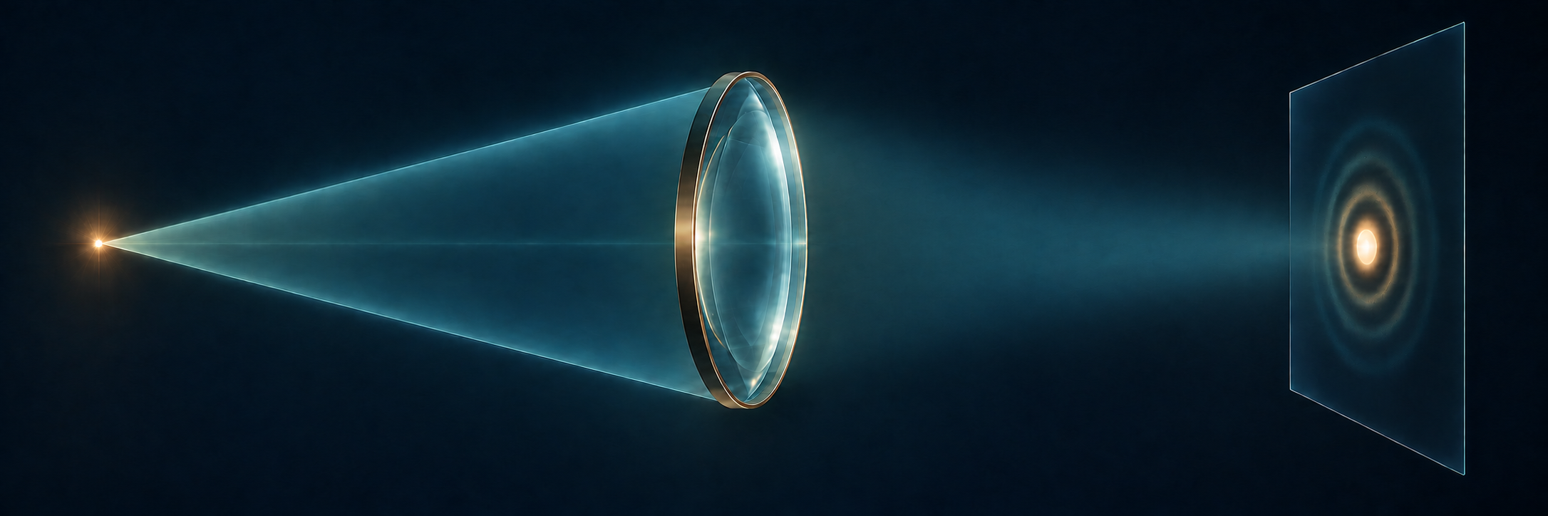
Calculate what a finite pupil does to a point, then judge which image details retain enough contrast.
The engineering question
An ideal lens brings rays from a distant point to its focal plane. Does that imply an infinitely small optical spot? If an image must retain at least 30% sinusoidal modulation at a specified spatial frequency, is removing geometric aberrations enough?
Section 2.3 introduced diffraction through the spreading and interference of light from an F-shaped aperture. Here we use the lens phase and propagation tools from Sections 2.2–2.3 to calculate one specified imaging system, then change its pupil. The resulting PSF and MTF extend the geometric image-quality framework in Section 1.6.
Model
An on-axis infinity-to-focus system in air
Begin with an on-axis object point at infinity, as in astronomical imaging. It supplies a uniform plane wave to an ideal thin lens at z=0 with focal length f>0. A circular aperture of radius a is immediately after the lens, and the sensor is at z=f. The aperture and lens share one plane in this thin-element model. The additional pupil masks introduced later occupy that same plane.
Use a monochromatic, scalar, paraxial field in air, so \lambda=\lambda_0 and k=2\pi/\lambda_0. Retain E(\mathbf r,t)=\operatorname{Re}\{U(\mathbf r)e^{-i\omega t}\}. Use x,y for physical transverse coordinates in each plane; z identifies the plane. At z=+f, they are sensor offsets from the on-axis geometrical image point. In propagation integrals, x',y' are dummy input-plane coordinates at z=0^+, while x,y are the observation coordinates. The image-space numerical aperture is \mathrm{NA}_{\mathrm i}=\sin\alpha\approx a/f. All PSF dimensions and intensity spatial frequencies below refer to this image space. High-NA vector focusing is outside this model.
This is a PSF for a declared object conjugate, pupil, wavelength, and sensor plane. Contributions from one object point add as complex fields. For mutually incoherent object points, their image intensities add. We use that latter condition for the intensity-convolution and MTF interpretation, within a small field where the point response is approximately shift invariant.
A distant point forms a finite focal pattern
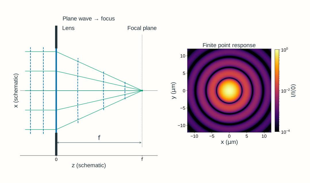
The incident wave is planar because the object point is at infinity. The ideal lens supplies the converging phase learned in Section 2.2. At the geometrical focus, contributions from the admitted aperture arrive with matching phase; at nearby sensor positions, their propagation phases differ. Their coherent sum gives a finite focal pattern rather than a geometric point.
Figure 2.13. A uniform plane wave from an on-axis distant point illuminates an ideal lens at z=0 with a circular aperture immediately after it. The sensor is at z=f. Here f=100~\mathrm{mm}, a=10~\mathrm{mm}, \lambda_0=600~\mathrm{nm}, and the paraxial image-space \mathrm{NA}_{\mathrm i}=0.10. Dashed curves are equal-phase wavefronts. Unequal schematic axis scales distort their apparent angles to the rays. The sensor-plane intensity map uses a logarithmic scale relative to its on-axis peak.
A clear circular pupil gives the Airy pattern
Follow the field from this one object point. Immediately before the lens, the plane wave has constant real peak electric-field amplitude (in V/m) E_0\ge0 and constant phase offset \phi_0:
U(x,y,0^-)=E_0e^{i\phi_0}
Choose the ideal lens’s center phase as zero. Its quadratic phase changes the wavefront, and the circular opening limits the admitted field. Immediately after both elements, inside x^2+y^2\le a^2,
On expanding the propagation phase, its input-coordinate quadratic term cancels the lens’s quadratic phase. The remaining sum is the circular-aperture Fourier transform already motivated in Section 2.3. Add these complex contributions first, then take the squared magnitude to obtain intensity.
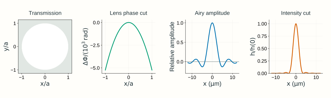
The circular-aperture transform gives the signed amplitude factor 2J_1(v)/v after separating the known propagation phase. Squaring its magnitude gives the Airy intensity pattern:
Here J_1 is the Bessel function of the first kind of order one; the ratio tends to one at the origin. This equation uses peak-normalized intensity only to describe the Airy shape. It is distinct from the unit-integral PSF normalization defined below.
Figure 2.14. The clear-aperture calculation for Figure 2.13’s infinity-to-focus system. The first panel shows amplitude transmission, not incident illumination; the illumination is uniform. The second shows the ideal lens’s actual quadratic phase relative to its center along y=0, using x/a on the horizontal axis and a scaled radian axis. Pupil maps use normalized coordinates x/a,y/a. The signed Airy amplitude factor is shown after separating the known propagation phase; squaring it gives the intensity shape. Both sensor-plane profiles are divided by their on-axis values, rather than normalized to unit integral.
To use this point response for image formation, normalize its intensity over the whole sensor plane:
This is Section 1.6’s normalized intensity PSF, with units of inverse image area. For mutually incoherent points in a small distant scene, shifted intensity PSFs add; each point’s angle sets its ideal focal-plane image position. This gives the same intensity-convolution interpretation used in Chapter 1, expressed in ideal image coordinates. Coherent points require field addition before taking intensity.
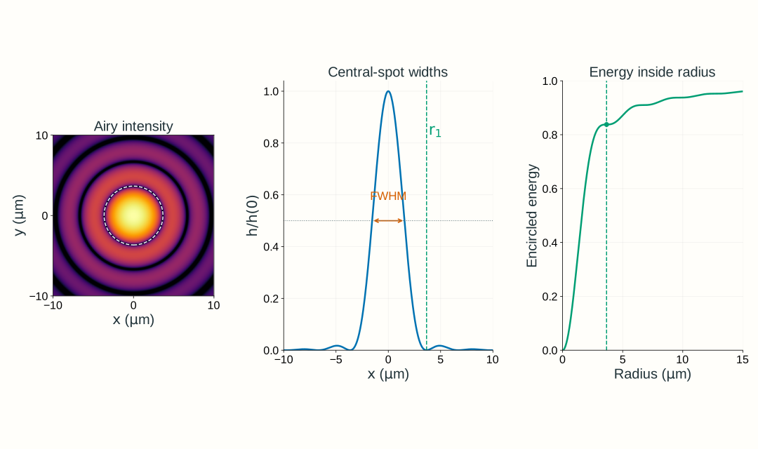
The first expression is a radius to the first dark ring; its diameter is twice as large. The second is the full width at half the central peak along a diameter. About 83.8% of the transmitted power lies within the first dark ring; the rest lies in the surrounding rings. Increasing NA or decreasing wavelength shrinks all these spatial scales, within the model’s validity.
Figure 2.15. For the infinity-to-focus system with its sensor at z=f, the clear circular pupil at 600 nm and image-space NA 0.10 has first-dark-ring radius 3.659 μm, central-peak intensity FWHM 3.087 μm, and 83.78% encircled energy within the first dark ring. The central disk is not a hard-edged container for all the light. The intensity map uses a logarithmic brightness scale to reveal rings; the central profile uses a linear vertical scale. Peak-normalized profiles describe shape; encircled energy refers to power integrated over area.Optional calculation: the circular-aperture transform
For this clear aperture, rotational symmetry reduces the remaining pupil integral to
Here \beta a=2\pi\mathrm{NA}_{\mathrm i}r/\lambda_0 under our paraxial NA convention. Retaining the full propagation phase, the sensor field for this particular lens-plane-to-focus calculation is
The input is specified at the lens plane, not the front focal plane. Propagation by f therefore retains e^{ikf} and the position-dependent output phase \exp[ik(x^2+y^2)/(2f)]. Section 2.3’s -f to +f transform instead has e^{i2kf} with no output quadratic phase; the coordinate names do not change these different geometries.
The phase factors have unit magnitude, so the intensity shape is [2J_1(v)/v]^2. The first positive zero is v\approx3.8317. Integrating intensity over a disk gives the encircled-energy fraction
\mathcal E(r)=1-J_0(v)^2-J_1(v)^2
This area integral, rather than a one-dimensional profile integral, determines the fraction of transmitted power inside radius r.
The intensity PSF determines diffraction-limited MTF
Recall Section 1.6’s relationship: the Fourier transform of the normalized intensity PSF gives the incoherent OTF, and its magnitude gives MTF. Here the PSF comes from diffraction rather than geometrical ray spreading:
Here \nu_x,\nu_y describe sensor-plane intensity variation, not the input field’s phase frequencies mapped to position in Section 2.3. This transform of an intensity PSF is different from Section 2.3’s transform of a complex input field. Because h integrates to one, \mathrm{OTF}(0,0)=1.
For the clear, uniformly illuminated, aberration-free circular pupil, the MTF is radial. Set \nu=\sqrt{\nu_x^2+\nu_y^2} and define
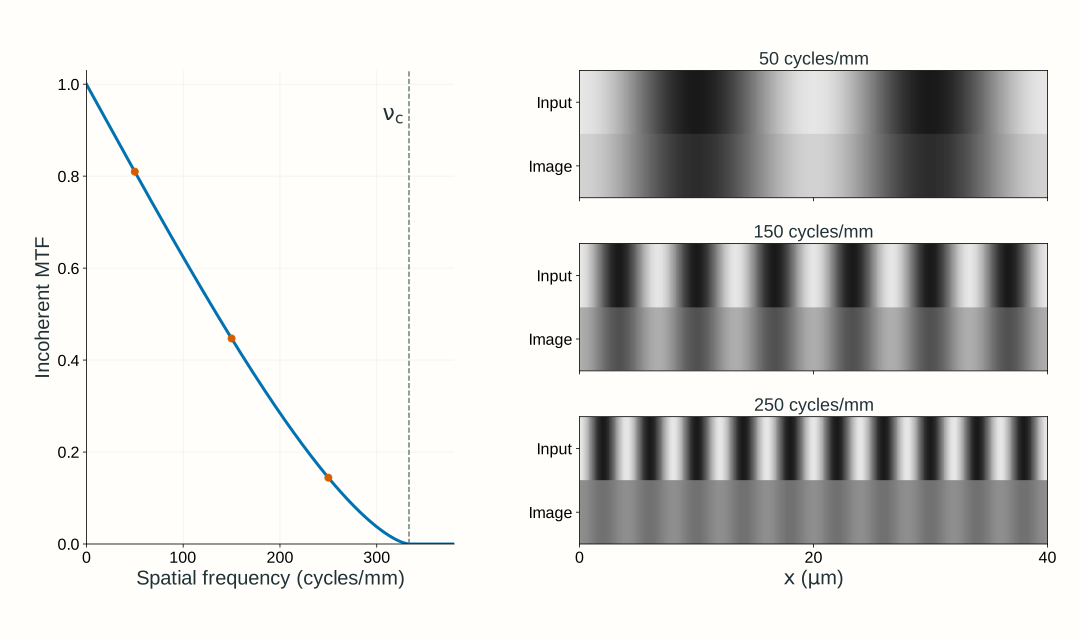
The MTF is zero beyond \nu_c. It approaches zero continuously at cutoff; frequencies merely being below cutoff does not guarantee useful contrast. At a given frequency, sinusoidal intensity modulation obeys m_{\mathrm{out}}=\mathrm{MTF}(\nu)m_{\mathrm{in}} under the declared incoherent, linear, locally shift-invariant model.
Figure 2.16. For the same infinity-to-focus system at 600 nm and image-space NA 0.10, the incoherent cutoff is 333.3 cycles/mm. The stripe comparisons use incoherent sinusoidal intensity input with modulation 0.80; the output modulation is that input modulation times MTF. All frequencies refer to the image plane. This does not apply the intensity MTF directly to the coherent field patterns in Section 2.3.
Why the incoherent cutoff is twice the coherent field cutoff
For ideal coherent imaging, the pupil transmits field components over a frequency disk of radius \mathrm{NA}_{\mathrm i}/\lambda_0. The incoherent OTF is a normalized autocorrelation of that pupil field. Two pupil positions can differ by a full pupil diameter, so the intensity-transfer support extends to 2\mathrm{NA}_{\mathrm i}/\lambda_0. These are different transfer functions for different illumination models, not two competing answers for the same bandwidth.
Optional explanation: pupil overlap gives the circular-pupil MTF
Shift one copy of the pupil relative to another. The normalized overlap integral of the pupil field with its complex conjugate is the OTF. A clear disk with no residual phase has equal positive contributions wherever the two disks overlap. Their overlap area, divided by the unshifted disk area, yields the circular-pupil MTF above. At a displacement equal to the pupil diameter, the overlap area vanishes. With phase error, the overlap integrand is complex, so contributions can cancel even where both pupils transmit.
Resolution depends on the question being asked
A spot-width number, a two-point criterion, and a stripe-contrast requirement answer different questions. A single point’s FWHM describes its central intensity profile. Rayleigh’s criterion places the peak of one equal-brightness, mutually incoherent Airy point at the other’s first dark ring, giving a reference separation \Delta x_{\mathrm R}\approx0.610\lambda_0/\mathrm{NA}_{\mathrm i}. It is not a universal detection threshold and does not describe arbitrary pupil shapes, unequal-brightness points, or coherent pairs.
For a quantitative imaging task, state the smallest relevant sinusoidal period, its input modulation, and the minimum acceptable output modulation. For this distant scene, small angular offsets map to focal-plane positions through x\approx f\theta_x; evaluate the corresponding intensity frequency in the sensor plane. For finite-distance objects, use magnification to convert object frequency to image frequency, as in Section 1.6. The calculation may reject a system well before its formal cutoff. Noise, detector response, and sampling impose additional requirements; Section 2.5 adds the camera and widefield design choices.
Change the complex pupil and repeat the calculation
Keep the same distant point, uniform incident plane wave, ideal lens, and sensor at z=f. Now replace the clear opening with a complex pupil immediately after the lens:
P(x,y)=t_p(x,y)e^{i\psi(x,y)}
The amplitude transmission t_p=|P| includes the circular opening and any attenuation; it is zero outside radius a. The phase \psi is additional to the ideal lens phase. It can represent a phase plate or a departure from ideal focusing. An optical-path difference W(x,y) gives \psi=2\pi W/\lambda_0. The incident plane-wave amplitude E_0 stays uniform; the transmitted amplitude E_0t_p(x,y) need not be uniform.
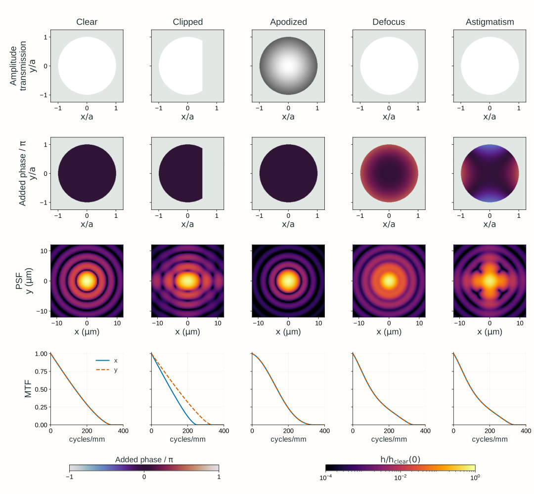
Repeat the same propagation calculation with this transmitted field: coherently add its contributions at the sensor, calculate |U(x,y,+f)|^2, normalize to obtain h, then Fourier-transform h to obtain OTF and MTF. Figure 2.17 shows the results of this calculation for five pupil choices.
Normalization describes where transmitted light goes, not how much survives the pupil. Report throughput separately: at fixed incident irradiance and aperture geometry, transmitted power is proportional to \iint E_0^2t_p(x,y)^2\,\mathrm dx\,\mathrm dy.
Clear pupil: the reference diffraction limit for this pupil geometry and uniform illumination.
Clipped pupil: removing a cap reduces throughput and makes the response direction-dependent. The nominal circular-pupil NA alone no longer describes its MTF.
Apodized pupil: gradual amplitude weighting reduces the influence of the edge. It can reduce rings while broadening the central response and reducing throughput; compare MTF at the task’s frequencies.
Defocus: an added quadratic phase moves the best focus relative to the fixed sensor at z=f. Moving the sensor can remove this defocus when the model permits.
Astigmatism: a phase term with different curvature along two transverse directions changes directional responses. One focus adjustment cannot make both curvatures ideal simultaneously.
These phase descriptions connect to Section 1.6’s aberration and refocusing diagnostics. A real prescription supplies a wavefront error and a transmitted pupil; a diffraction calculation then adds those pupil fields. A geometric spot diagram remains useful, but cannot replace that coherent sum.
Figure 2.17. Pupil changes in the same infinity-to-focus system: a uniform plane wave, an ideal lens, the complex pupil immediately after it, and a fixed sensor at z=f. The wavelength is 600 nm and reference image-space NA is 0.10. The first row is amplitude transmission t_p, not incident amplitude. The second row is the added phase \psi; the ideal lens phase is not plotted. Clipping removes the cap x/a>0.5; apodization uses t_p=e^{-\rho^2} inside the disk, where \rho^2=(x^2+y^2)/a^2. Defocus adds edge-to-center optical-path difference 0.25 waves while the sensor remains at the reference focal plane; astigmatism uses \psi=2\pi(0.25)[(x/a)^2-(y/a)^2]. PSFs are normalized over the whole calculation plane, not the displayed crop; throughput is reported separately relative to the clear pupil. The PSF maps share one logarithmic brightness scale relative to the clear pupil’s unit-integral PSF peak. Directional MTFs are normalized at zero frequency. Phase-only changes preserve admitted power but can reduce contrast. The balanced astigmatism shown here has matching x and y MTF cuts at this plane; clipping illustrates different directional responses.
Explore: change the pupil and inspect image quality
Use the same plane-wave → ideal lens → complex pupil → fixed focal-plane sensor setup. Choose a pupil, then change wavelength, image-space NA (the ratio a/f), and the added phase strength where applicable. Compare amplitude transmission and added phase with the intensity PSF, its central profiles, and directional MTF. Keep track of relative throughput as well as normalized image quality. The displayed first-dark-ring radius and cutoff are clear circular-pupil reference scales, not universal measures for the altered pupils.
Model, numerical method, and validation
The explorer models an on-axis point at infinity: a uniform plane wave, ideal focusing lens, immediately adjacent pupil, and sensor at the reference focal plane. It uses scalar paraxial propagation in air. Defocus changes the added pupil phase; it does not move the sensor or introduce a finite-distance object. Its pupil panels use x/a,y/a, normalized to the reference circular radius, while the sensor panels show physical x,y at z=+f. The clipped, apodized, defocused, and astigmatic presets use the definitions in Figure 2.17. Phase strength is measured in vacuum-wavelength optical-path waves at the selected wavelength; changing wavelength with this strength held fixed therefore changes the specified physical path error.
The ideal lens phase cancels the input quadratic phase in Fresnel propagation to z=f. A padded two-dimensional FFT then sums the transmitted amplitude and added phase. Known output phase factors do not affect intensity, and their uniform magnitude scale cancels in PSF normalization. Its squared magnitude supplies the intensity PSF; whole-grid normalization separates spatial redistribution from throughput. Directional MTFs come from the pupil autocorrelation, with padding chosen to avoid circular overlap. Spatial plots use fixed physical axes and one declared reference intensity scale. The displayed field of view can miss PSF energy; that omitted fraction is reported rather than renormalized away.
Analytical Airy widths, circular-pupil MTF, pupil-power integrals, phase-only throughput conservation, and grid refinement check the calculation. The standalone explorer retains its full model explanation and a static fallback. These teaching examples do not establish Lab 2 software requirements.
An instructor-side check also exercises Optiland 0.6.3’s real-surface wavefront, FFT PSF, and FFT MTF analyses for Chapter 1.6’s singlet geometry at 600 nm. Independently reconstructing its exported complex pupil with NumPy reproduces the normalized PSF and MTF; pupil refinement changes MTF at 40 cycles/mm by about 0.0012. This checks the exercised diffraction workflow, rather than independently certifying the underlying ray tracing or optical-path calculation. The browser explorer uses controlled pupil functions to isolate amplitude and phase effects.
What changes for a finite-distance object?
A PSF belongs to a specified object conjugate and sensor plane. For an on-axis object point at a finite coordinate z_o<0, replace the plane-wave input with the spherical wave from that point. Apply the lens and pupil transmission, then propagate the resulting field to the selected sensor plane. The wave tools are unchanged; the incident amplitude and phase, image-space NA, and any real-lens aberrations must match the new configuration.
Use Chapter 1’s signed imaging relation to locate the paraxial image conjugate. With the same ideal lens and aperture, an object at z_o=-2f is imaged at z_i=2f. Refocusing the sensor there halves image-space NA from approximately a/f to a/(2f). Under the ideal, nearly uniform pupil-illumination approximation, the in-focus pattern is still Airy-shaped, but its first-dark radius and FWHM double in physical sensor coordinates and its incoherent cutoff halves. Keeping the sensor at f would instead leave the finite-distance point defocused.
Thus refocusing does not, by itself, preserve the PSF size. For finite-distance objects use the corresponding magnification when relating object detail to image detail. The preceding figures and explorer hold the infinity-to-focus conjugates fixed to isolate pupil effects; a real finite-conjugate system needs its own point-response calculation.
Worked examples
Guided
State which spot width you mean
A uniformly illuminated, clear circular pupil forms a scalar paraxial image in air at \lambda_0=600~\mathrm{nm} with image-space \mathrm{NA}_{\mathrm i}=0.10. Find the first-dark-ring radius, its diameter, and the central intensity FWHM. Would a 3 μm diameter disk contain most of the transmitted power?
Hint / setup
Use one length unit, distinguish radius from diameter, and compare the proposed disk’s radius with the Airy scales. Encircled power is an area integral, not the intensity at the disk’s edge.
Full solution
\frac{\lambda_0}{\mathrm{NA}_{\mathrm i}}=\frac{0.600~\mu\mathrm m}{0.10}=6.00~\mu\mathrm m
r_{\mathrm{dark},1}=3.659~\mu\mathrm m,\qquad 2r_{\mathrm{dark},1}=7.318~\mu\mathrm m,\qquad d_{\mathrm{FWHM}}=3.087~\mu\mathrm m
A 3 μm diameter disk has radius only 1.5 μm, slightly less than the half-maximum radius. It therefore does not enclose most of the power. The exact circular-pupil encircled-energy expression gives about 45.6% within that radius; the larger 7.318 μm diameter Airy disk encloses about 83.8%. A FWHM is not an energy-containing diameter.
Scaffolded
A frequency below cutoff can still fail a contrast requirement
Use the same clear pupil and wavelength. An incoherent sinusoidal intensity pattern has image-space frequency 150 cycles/mm and input modulation 0.80. Find the cutoff and predicted output modulation. Does the system meet an output-modulation requirement of at least 0.40?
Hint / setup
Convert 600 nm to mm, calculate \nu_c=2\mathrm{NA}_{\mathrm i}/\lambda_0, then evaluate the circular-pupil MTF at q=\nu/\nu_c. Apply the modulation ratio, not the amplitude of a coherent field.
The frequency is below cutoff, yet 0.3576 is less than the required 0.40. This ideal diffraction-limited system fails that contrast requirement. Merely reporting a cutoff or an Airy diameter would miss this decision.
Independent
Choose a pupil against contrast and throughput requirements
At 600 nm, compare three ideal, aberration-free pupils under the same uniform incident irradiance: the clear reference pupil with image-space NA 0.10; a concentric stopped pupil with NA 0.075; and the original NA 0.10 disk with amplitude transmission t_p=e^{-\rho^2}. For incoherent image-space stripes at 150 cycles/mm with input modulation 0.80, require output modulation at least 0.30 and at least 60% of the clear reference pupil’s transmitted power. Which configuration meets both?
Hint / setup
For the stopped clear pupil, throughput scales with pupil area and its MTF uses the reduced NA. For the apodized pupil, power transmission depends on t_p^2, not t_p. Use its numerically evaluated MTF below; the clear-disk MTF formula does not apply after amplitude weighting.
The apodized MTF is evaluated by the normalized pupil-overlap integral with the same image-space frequency and reference NA.
Full solution
Pupil
Relative throughput
MTF at 150 cycles/mm
Output modulation
Meets both?
Clear, NA 0.10
1.0000
0.4470
0.3576
Yes
Stopped, NA 0.075
0.5625
0.2848
0.2278
No
Apodized, reference NA 0.10
0.4323
0.4440
0.3552
No
The stopped pupil has throughput (0.075/0.10)^2=0.5625 and cutoff 250 cycles/mm; it fails both requirements. Apodization meets the modulation requirement at this frequency but fails throughput. Only the clear pupil meets both. Reducing rings or stopping down is not an improvement by itself; judge each change against the stated task. The comparison holds incident irradiance fixed, rather than compensating losses by increasing illumination.
Model selection and engineering checks
Specify the imaging configuration. Declare the object distance and field point, lens and pupil, wavelength, and sensor plane. The figures and explorer use an on-axis point at infinity and a sensor at the ideal lens’s reference focal plane; finite-conjugate PSFs require the corresponding incident wave and image-space NA.
Identify the illumination model. Coherent field addition across one pupil and incoherent intensity addition across independent object points are different steps. Apply the intensity MTF only under its stated imaging assumptions.
Match the space and wavelength. Use image-space NA with image-space dimensions and frequencies. With NA defined as n\sin\alpha, the formulas use vacuum wavelength; with pupil geometry and k, use wavelength in the medium.
Keep normalization explicit. Unit-integral PSF, peak-normalized Airy shape, zero-frequency-normalized MTF, and relative throughput are not interchangeable quantities. Do not normalize a cropped PSF to hide missing energy.
Check direction, field, and focus. Asymmetric pupils and aberrations can give different MTF curves along different directions. A central-field curve is not a guarantee over the whole field of view.
Check limiting cases. A clear pupil recovers Airy widths and circular-pupil MTF. A uniform phase changes no intensity; phase-only pupil changes preserve transmitted power. Clear-pupil MTF starts at one and vanishes at its cutoff.
Check numerical convergence. Resolve the pupil edge and phase variation, pad the field transform, and refine pupil sampling. Ensure autocorrelation is not wrapped by periodic boundaries. Compare PSF widths, energy, and directional MTF with analytical or independently integrated references.
Check the physical model. At high NA, vector polarization, exact focusing geometry, and nonuniform illumination can invalidate scalar paraxial predictions. Real-lens diffraction analysis must use the actual transmitted pupil and wavefront at a declared reference focus.
Section 2.5 combines these optical bandwidth and contrast limits with camera sampling, pixel integration, field coverage, and through-focus design choices.