Depth of field and field of view

The engineering question

How much of a specimen can we image, laterally and axially, for a specified sensor, aperture geometry, and acceptable blur? A point can be sharply focused but vignetted, or fully transmitted but defocused. We need separate checks for blur, sensor coverage, and bundle transmission.

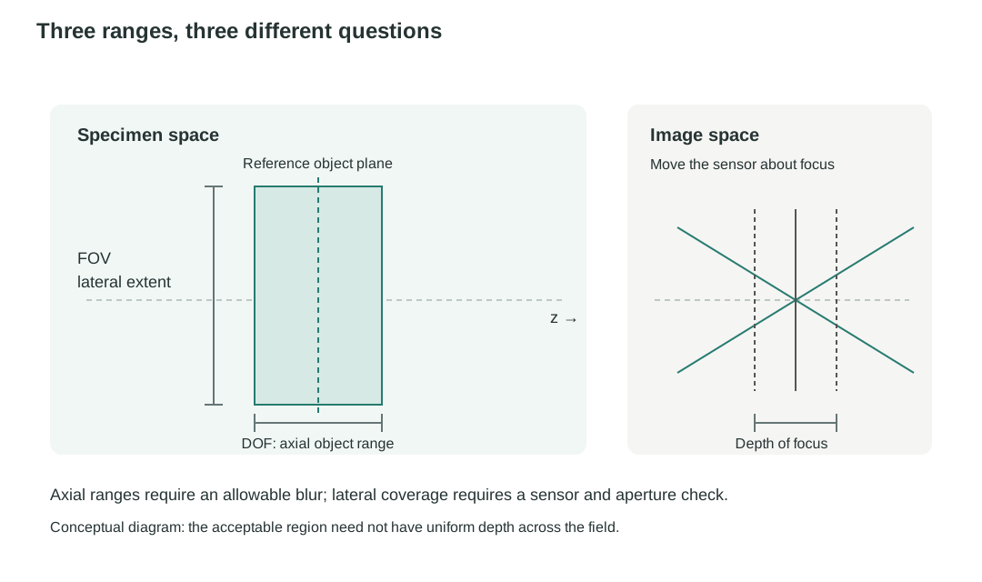
Three ranges, three different questions

A displaced sensor turns a cone into a blur disk

Begin with the single-thin-lens imaging example from Chapter 1.2, taking the lens opening as the aperture stop and an on-axis object point. With no optics after the lens, the exit pupil coincides with that opening. We use this setup through Figure 1.15. At the ideal image plane, the imaging condition sends rays from the object point to the same height . Move a sensor by from that plane. Free propagation gives

Thus, a finite range of image-side slopes becomes a finite disk on the displaced sensor. If is the image-side half-cone angle, the geometric sensor-plane blur-disk diameter is

For a general imaging system, including one with several lenses, the same blur-diameter relation applies to the actual image-side cone. As explained in Chapter 1.4, its half-angle is determined by the exit pupil’s diameter and axial distance from the ideal image point. The final lens diameter alone does not generally determine this angle, because the exit pupil can differ from that lens in both size and position. The following discussion uses this general image-side cone.

Choose an allowable blur disk: the circle of confusion

Here is the geometric blur-disk diameter at the sensor. Choose a task-specific maximum : the conventional photographic name for this chosen limit is the circle of confusion. It is a requirement for acceptable performance, not a universal optical constant.

• Sensor-pitch criterion: choose a stated limit relative to pixel pitch, such as one pixel pitch or a justified fraction of it.
• Object-feature criterion: a required object-space feature of size maps to at the sensor. Choose as a stated allowable fraction of that mapped feature size.

Choose to meet the imaging task’s requirements, leaving room for other sources of blur and error in the complete imaging system.

The pupil controls depth of focus

In the paraxial approximation, the one-sided sensor tolerance that keeps is

This is the half-range of geometric depth of focus; a symmetric total depth of focus is twice this value. A wider image-side cone makes the sensor tolerance smaller.

The image-side numerical aperture, , describes this cone, where is the refractive index in image space. Here we assume air between the last lens and the sensor, so . For paraxial rays, , and the total geometric depth of focus is

The image-side working f-number describes the same actual cone. As explained in Chapter 1.4, in air and in the paraxial approximation, . Thus,

For a focusing system in air with the object at infinity, the working f-number approximately equals the nominal f-number , where is the effective focal length and is the entrance-pupil diameter.

Stopping down (reducing the aperture stop diameter) therefore increases geometric depth of focus. It does not by itself establish resolution, because diffraction is not included in this model.

Depth of field is the corresponding object-side range

Depth of field (DOF) is the allowed object-side axial range while the lens and sensor stay fixed. Moving the object shifts its ideal image plane away from the sensor, so the sensor intercepts a blur disk. The near and far object positions where that disk reaches bound the acceptable range.

A local estimate from depth of focus

Consider a thin lens in air on both sides. At the reference focus, the object is at and its image is at the fixed sensor, . The transverse magnification there is . Differentiating the signed thin-lens relation gives

Here is a small object displacement from reference focus, and is the resulting displacement of its ideal image plane. The sensor remains at . Its separation from the displaced ideal image plane has magnitude , which must stay within the one-sided depth-of-focus tolerance. Therefore, the total object-side range is approximately

Evaluate the image-side numerical aperture and working f-number at the reference focus. This estimate assumes a small enough object range that the magnification and image-side cone change little. The same local axial magnification holds for a fixed compound paraxial system in equal object and image media: its imaging matrix has determinant one, giving axial magnification equal to the square of transverse magnification. For the same sensor blur criterion and image-side cone, larger magnification makes the acceptable object-depth range smaller.

Express DOF using objective NA

For microscopy, it is often more convenient to use the object-side numerical aperture, , commonly called objective NA. In paraxial imaging with air on both sides, transverse magnification and angular spread change inversely: magnifying the image by narrows the image-side cone by the same factor. Thus, . This relation follows from Chapter 1.2’s imaging matrix and also holds for compound lens systems. Both NAs must describe the same transmitted ray bundle; additional apertures can reduce the admitted NA below the objective’s rated value.

Substituting into the local estimate gives the total geometric depth of field in air:

Here is the total magnification from the specimen to the sensor where is specified. Alternatively, define the object-equivalent allowable blur diameter as . Then

For a fixed allowable blur expressed in specimen space, a larger objective NA gives a smaller geometric DOF. These remain local, paraxial estimates around reference focus. Chapter 2 will introduce diffraction and its wavelength-dependent contribution to the acceptable focus range.

This is geometric depth of field for a chosen blur criterion. Object-space telecentricity, introduced in Chapter 1.4, can stabilize image scale as the object moves axially, but it does not eliminate the defocus blur that limits this range.

Sensor size gives a first estimate of field of view (FOV)

At the reference object plane, a lateral height maps to image height . If the sensor has full active width , the corresponding full object-field width and half-field are

This is a sensor-limited candidate field: it tells us which object points would have focused images on the sensor. Here is a full width in object space, whereas is the physical sensor width. We still need to check whether the optics transmit the required ray bundles from those points. The magnitude of magnification sets width; its sign sets image orientation. For a distant scene, field is instead often specified as an angle. That angular field must be mapped through the system; it is not the same quantity as a finite specimen width in millimeters.

A focused point whose image lies on the sensor may still lose some or all of its rays at an earlier aperture. Increasing sensor width cannot recover rays already blocked by the optics. The next step is therefore to find how much of this candidate field is transmitted without clipping.

Which opening sets the field?

Chapter 1.4 compared candidate openings to find the aperture stop: the opening that limits the ray cone from an on-axis object point. We can make a parallel comparison for the field. In the simplest geometric case, place candidate openings at object-conjugate image planes. Rays from each object point meet at one position in each such plane, so an opening there selects object locations rather than narrowing the cone from an admitted point. The opening that gives the smallest object-space field is the field stop. A field stop need not lie at an object-conjugate plane; placing it there produces a sharp geometric field boundary. Its role depends on both its size and where the optics form the images, not on whether the hardware is called an iris, diaphragm, or aperture.

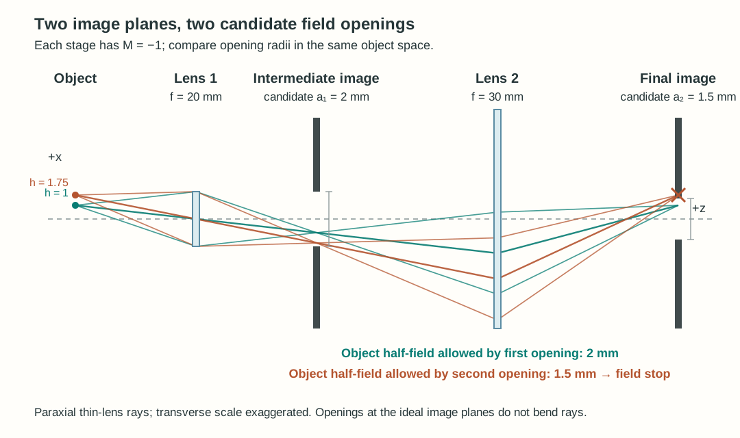
For example, let lens 1 form an intermediate image with transverse magnification , then let lens 2 image that plane onto a final image plane with . This is a sequential two-lens imaging system: the plane between the lenses is an intermediate object image, not the Fourier plane between the lenses of the 4-f relay in Chapter 1.3. Put a candidate opening of radius at the intermediate image and another of radius at the final image. In the illustrated model, lens 1 has a clear radius of and sets the on-axis cone; lens 2 has a clear radius of and passes those admitted bundles over the fields considered.

Both candidates are measured against the same object height . The second opening is more restrictive, so it is the field stop in this example. A point at passes both; a point at passes the intermediate opening but is blocked at the final one. In the ideal ray model, reducing an opening at an exact image plane leaves the on-axis ray cone intact as long as its center remains open. A finite real spot requires an additional image-quality check.

The active sensor boundary can also limit which field is recorded. An opening away from an image plane instead meets a ray bundle of finite width: as field height grows, it can start blocking some rays before it blocks the whole object point. That gradual loss leads to vignetting.

Vignetting can reduce the fully transmitted FOV

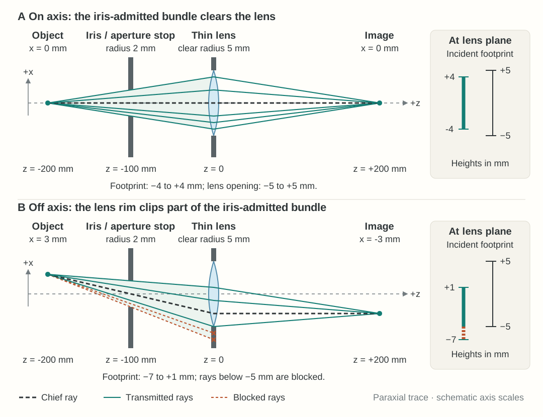
Follow the entire ray bundle from one object point. As we learned, object-side NA characterizes the accepted ray cone leaving that point, while image-side NA characterizes the converging cone at its image point. Between these two ray cones, the bundle generally has a finite width that varies through the system. Its cross-section at a specified surface or plane is called the bundle footprint. For an off-axis object point, this footprint can shift toward the edge of a lens or opening—not necessarily the aperture stop. If part of the footprint falls outside the clear opening, those rays are blocked while the remaining rays pass. This partial loss is called vignetting. The chief ray may still pass, so checking it alone does not establish that the whole bundle is transmitted.

For a circular bundle of radius centered a distance from a circular opening's axis, with clear radius , full transmission requires

Partial overlap occurs when ; at there is no finite-area overlap. These conditions describe the simple circular footprints used below. More general bundles require their actual footprints. A few drawn rays illustrate clipping but do not establish transmitted power.

In this section, a design passes the aperture-clearance check only if the entire ray bundle admitted by the aperture stop from every required object point clears the remaining optics. Partial clipping fails this requirement, even though the surviving rays can still form an image of that point. Some applications allow a specified amount of light loss, but the examples below use the stricter requirement of no clipping.

The fully transmitted field is the range of object points whose entire stop-admitted bundles clear the optics, before applying the sensor boundary. Under our no-clipping requirement, the usable field must satisfy both optical transmission and sensor coverage. For centered, symmetric fields at the reference focus, their full object-space widths obey

Here is the fully transmitted optical width. All three widths in this equation refer to the same object plane and transverse direction. A partially vignetted point may still be recorded outside this usable field; it simply fails our no-clipping requirement. The edge of the fully transmitted field marks the onset of clipping, not necessarily a sharp boundary beyond which the image disappears.

Changing lens spacing can increase the usable FOV

Consider an ideal infinity-corrected microscope. The objective has at ; the reference specimen is at . A circular stop of diameter lies at the objective's rear focal plane, . A tube lens with is at , and the sensor is at . Give the objective and tube lens clear radii of ; there are no other limiting openings.

Label specimen height by and a ray's stop height by . These are different coordinates: chooses the object point, while chooses a ray within its bundle. At reference focus, the objective produces slope . Propagating from the stop to the tube lens gives

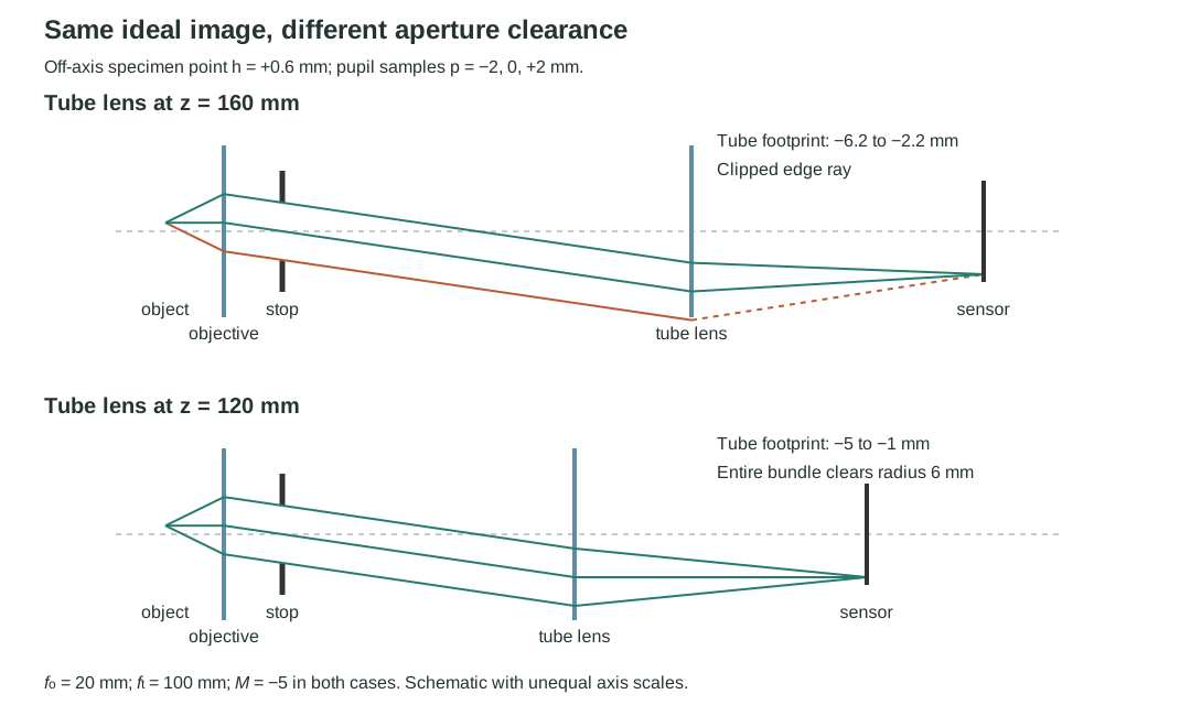
The tube-lens footprint radius is , but its center shifts by when and by when . Moving the tube lens and its sensor together preserves ideal reference-plane focus and , while reducing the footprint displacement.

Now give the sensor a full width of . Both spacings have . The tube-lens clearance conditions are for the longer spacing and for the shorter spacing. These give fully transmitted half-fields of and , respectively. The objective is nonlimiting over both optical fields: its footprint obeys .

At the longer spacing, vignetting reduces the no-clipping usable FOV below the sensor-limited estimate. Moving the tube lens and sensor together reduces the off-axis footprint displacement, so the optics transmit the entire sensor-limited field at the shorter spacing. The image scale and sensor coverage stay the same, but the usable width increases from about to . Further increases in optical field alone would not enlarge the field recorded by this sensor.

Explore: lens spacing and field of view

Keep the object point at the sensor-field edge and shorten the lens spacing. Find where the full optical field first covers the sensor field, then move the object point to compare the two limits.

This comparison applies to the reference object plane, where ideal point images are focused on the sensor. A specimen with finite thickness also produces defocus blur. The final worked example checks whether that blur still fits on the sensor at the combined field and depth extremes.

The rear-focal-plane stop makes this model object-space telecentric. It stabilizes chief-ray image scale under small specimen displacements with this fixed sensor configuration. It does not eliminate defocus, aperture clipping, or blur extending beyond a sensor edge.

Worked examples