Describe a field as spatial-frequency components, map them with a lens, and change the reconstructed field with an amplitude or phase mask.
The engineering question
Place a small mask between the lenses of a 4-f relay. Why can that mask change the image even though it is not in an image plane? A lens separates tilted plane-wave components by position at its focal plane. The mask can then transmit, block, or phase-shift selected components before a second lens combines them again.
Section 2.2 supplied lens phase and paraxial propagation. Fourier optics organizes those same field operations by spatial frequency. We reuse Chapter 1’s relay geometry; calculating diffraction PSFs and incoherent MTF is the next step in Section 2.4.
Model
A monochromatic, coherent, paraxial model
We model one electric-field component in a homogeneous, transparent, nonmagnetic medium. The field is monochromatic and coherent, with the same convention as Section 2.1:
Here A=|U|\ge0 and \Phi are real wherever the field is nonzero. Retain the full spatial field U, including its axial phase. The wavelength in the medium is \lambda=\lambda_0/n, and k=2\pi/\lambda. Use consistent length units; spatial frequencies \nu_x,\nu_y are in cycles per unit length, such as cycles/mm, while f denotes focal length.
Use forward paraxial propagation and ideal thin lenses in the same medium. Complex fields add before intensity is calculated. Finite lens apertures, vector effects, and high-angle propagation require additional checks; the ideal lens Fourier mapping below explicitly assumes no lens clipping.
A tilted plane wave represents one spatial frequency
A plane wave’s phase can be written
\Phi(x,y,z)=2\pi(\nu_xx+\nu_yy)+k_zz+\phi_0
One cycle of transverse phase corresponds to 2\pi radians. Thus k_x=2\pi\nu_x and k_y=2\pi\nu_y. Section 2.2’s local angle expression becomes
\theta_x\approx\frac{k_x}{k}=\lambda\nu_x
A positive \nu_x gives an upward tilt; a negative one gives a downward tilt. For a nonzero one-dimensional component, the transverse phase period is d=1/|\nu_x|. These are spatial cycles along a plane, not the temporal oscillation frequency: all components here share the same \omega.
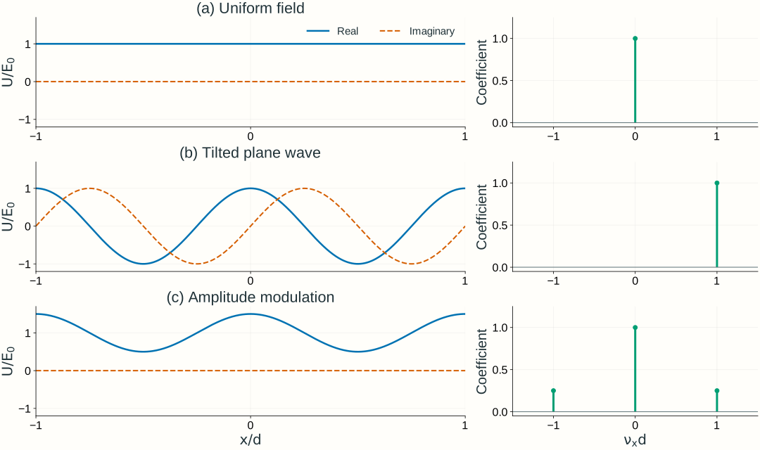
A single tilted plane wave has constant intensity even though its phase varies across the plane. A real amplitude pattern such as 1+m\cos(2\pi\nu x) instead contains three components: a constant term and waves with frequencies +\nu and -\nu. The cosine is an amplitude modulation, not a detected intensity pattern.
Figure 2.8. Different fields require different spatial-frequency components. Solid and dashed curves show real and imaginary field parts. The three examples are U/E_0=1, e^{i2\pi x/d}, and 1+0.5\cos(2\pi x/d). The right panels show dimensionless coefficients of these ideal periodic components, rather than the units or finite widths of a continuous Fourier spectrum. All plotted coefficients happen to be real; general coefficients are complex.
A general field combines spatial-frequency components
The Fourier transform finds the complex coefficient of each tilted component at a chosen plane. With a negative exponential for the forward transform and dummy integration coordinates x',y' at that plane,
Each coefficient carries magnitude and phase. Keeping only the spectrum’s magnitude loses information needed to reconstruct the field. If lengths are in mm, \widetilde U has field units times mm², and the inverse transform integrates over inverse area to recover field units.
For the simple periodic pattern in Figure 2.8, a finite sum makes the idea transparent:
Here E_0\ge0 is a real field scale in V/m, not necessarily the pattern’s peak amplitude. Constant fields and infinite plane waves have delta-function spectra in the continuous transform; the finite sum uses their discrete coefficients directly. A finite illuminated pattern instead has broadened spectral features.
Transform the complex field, then calculate intensity. The field spectrum is not the Fourier transform of intensity. In particular, the square-law detector creates cross terms between components; it does not simply display their separate powers.
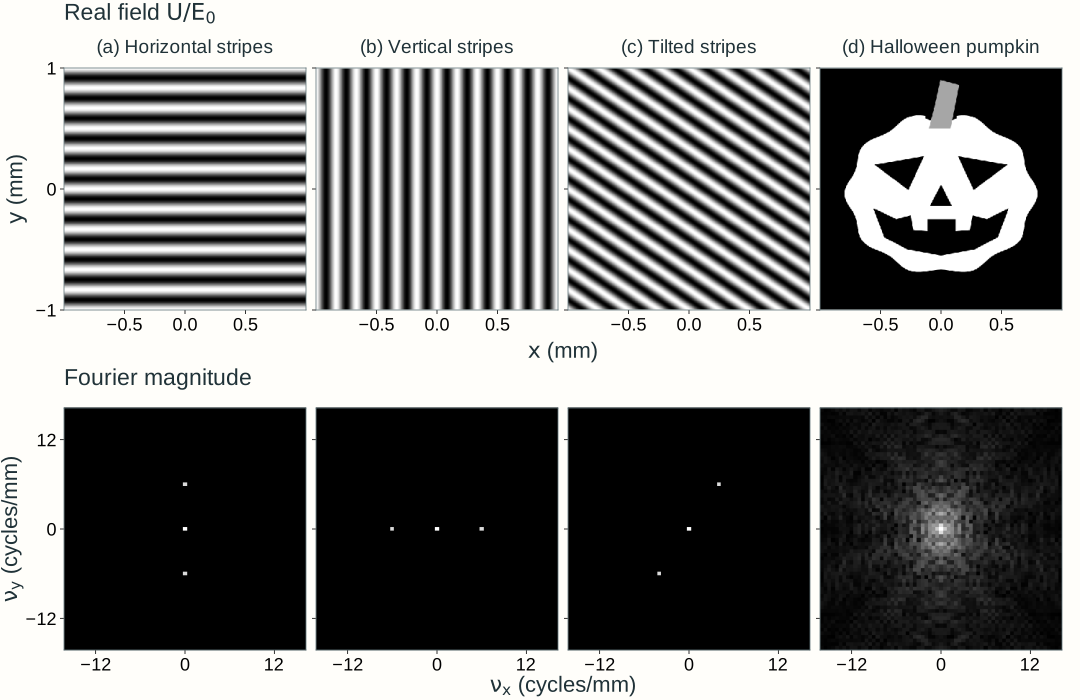
In two dimensions, stripe orientation determines where the paired components lie in (\nu_x,\nu_y): the frequency vector is perpendicular to the stripes. A more detailed pattern, such as the pumpkin in Figure 2.9, combines many spatial frequencies. Here we assign each grayscale pattern to a real, nonnegative field amplitude with uniform phase; we transform that field rather than a measured intensity image.
Figure 2.9. Two-dimensional patterns and their field spectra. Horizontal stripes vary along y, vertical stripes along x, and tilted stripes along both coordinates. Each sinusoid has a zero-frequency component and two opposite-frequency components, at (0,\pm6), (\pm6,0), and \pm(4,6) cycles/mm, respectively. The pumpkin’s outline and facial details require a broader range of frequencies. Top row: U/E_0, from black (0) to white (1). Bottom row: Fourier magnitude, normalized separately for each spectrum and logarithmically compressed to reveal weaker components; brightness is not optical intensity, and spectral phase is not shown. The sinusoidal patterns repeat across the sampled window; the pumpkin is zero outside its silhouette. Only the central frequency region is displayed.
Explore: build a pattern from spatial frequencies
Choose an input pattern, select low-pass or high-pass filtering, and adjust the circular cutoff to see which details remain after reconstruction. Click the spectrum to inspect a frequency pair, or enter its coordinates. Selecting a component changes the sinusoidal preview; it does not change the filter. The panels show electric-field values, not intensity.
Model, numerical method, and validation
The input is a real, nonnegative field U/E_0 with uniform phase. A two-dimensional FFT decomposes a 2 mm square into discrete components on a 256 × 256 grid, with frequency spacing 0.5 cycles/mm. The spectrum panel shows only the central region, |\nu_x|,|\nu_y|\le16 cycles/mm. Its logarithmic magnitude display reveals weak components; the calculation retains their complex phases.
Low pass (the default) retains components with \sqrt{\nu_x^2+\nu_y^2}\le\nu_c, including the boundary; high pass retains the complementary components outside the circle. High pass removes the DC component, leaving a zero-mean signed field. Pass all removes the cutoff and includes every sampled component, including those outside the displayed spectrum. Moving the cutoff slider or changing the filter type restores circular filtering. The output is the inverse FFT of the masked complex coefficients, without the inversion or common phase of a physical 4-f relay.
Real fields have conjugate coefficients at opposite frequencies. For a discrete coefficient c of the normalized field U/E_0, their combined normalized contribution is
b(x,y)=2|c|\cos[2\pi(\nu_xx+\nu_yy)+\arg c]
The lower-middle panel divides this contribution by its amplitude for visibility and reports the actual amplitude separately. Zero frequency contributes a constant and is counted once. A negligible coefficient has no meaningful phase preview. The opposite-frequency marker identifies the partner; the selected pair remains inspectable even when the cutoff excludes it.
The FFT treats the computational square as periodic. The stripe patterns repeat across its edges; the pumpkin and geometric pattern have a dark margin. Filtering can spread field values to the boundary, so this finite periodic calculation is not an infinite-domain propagation model. A sharp cutoff can also produce ringing and negative field values. Input and output share a fixed signed field scale; no per-image contrast normalization is applied.
Checks compare the browser calculation with an independent NumPy FFT, including full-pass reconstruction, DC-only output, known stripe frequencies and coefficients, conjugate symmetry, selected-pair phase, and Parseval’s relation. Complementary low-pass and high-pass outputs sum to the original field. Grid-refinement checks assess the finite pattern’s sampling. The existing 4-f explorer below separately connects filtering to lens geometry; neither explorer defines Lab 2 software requirements.
Propagation changes the phase of each component
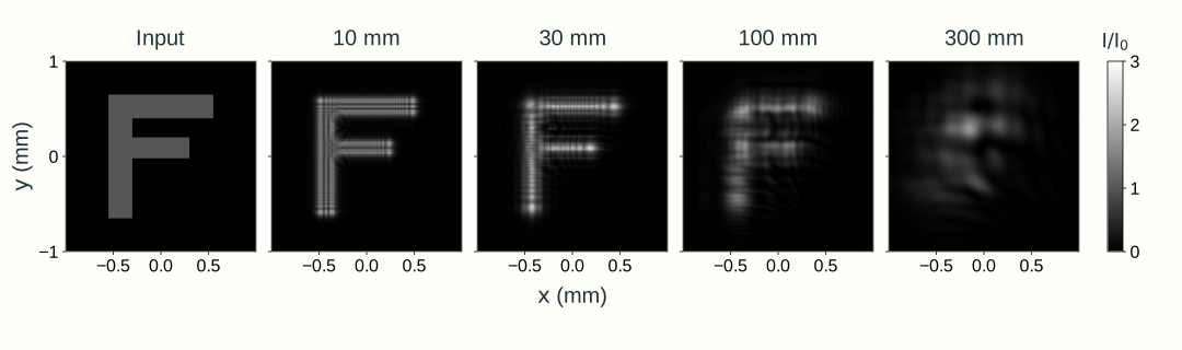
Imagine the explorer’s input letter F as a thin F-shaped opening in an opaque screen. A broad, coherent, monochromatic plane wave illuminates it with nearly uniform amplitude and flat phase. Immediately after the opening, the transmitted field has the F shape and a common phase wherever it is nonzero. As it propagates downstream without a lens, light spreads beyond that geometric outline and contributions from different parts of the opening interfere. This spreading and interference of a finite field during propagation is diffraction.
Section 2.2’s Fresnel integral calculates this evolution by adding contributions from input-plane patches. We can express the same propagation in the spatial-frequency domain, where each plane-wave component acquires a propagation phase. For propagation by L>0 through the common medium,
The quadratic phase depends on spatial frequency, so propagation changes the relative phases of the components. Recombining them produces edge fringes and redistributes the F’s intensity. The propagated field U is generally complex; a detector measures intensity proportional to |U|^2. The common axial factor e^{ikL} remains part of U and cancels from intensity.
This equivalent calculation follows transform → multiply by H_L → inverse transform: decompose the input field into spatial-frequency components, apply each component’s propagation phase, and recombine them. The upstream explorer’s low-pass or high-pass mask removes components; free-space propagation instead has |H_L|=1, preserving every component magnitude while changing phase. Ideal propagation conserves full-plane power within this model. A finite numerical or detector window can miss redistributed light.
For the F’s approximately 220–250 µm bar widths, 600 nm light in air propagated by 1 mm has a characteristic edge-diffraction scale \sqrt{\lambda L}\approx25~\mu\mathrm m. The outline remains recognizable while fine fringes develop near its edges. Increasing distance progressively redistributes the pattern, with no sharp distance at which its shape disappears. Figure 2.10 compares longer propagation distances on fixed spatial and intensity scales.
Figure 2.10. Diffraction after an F-shaped aperture. A broad, coherent plane wave at 600 nm in air illuminates the ideal thin opening. The input and downstream panels share the same 2 mm square viewing window and intensity scale I/I_0=|U/E_0|^2, where I_0 is the incident intensity. Labels give propagation distance L. Scalar paraxial fields are calculated from analytical rectangular-aperture Fresnel integrals, and each map uses area-averaged intensity samples. Increasing distance changes component phases and redistributes intensity while preserving the full field’s power. Light outside the displayed window is omitted from the picture.
Section 2.4 applies this diffraction physics to a finite pupil and a lens: the focal point response leads to the intensity PSF, MTF, and resolution limits.
A lens maps spatial frequency to focal-plane position
Place an ideal lens at z=0. Specify the input field U(x,y,-f) in the front focal plane and observe U(x,y,+f) in the back focal plane. Use the same transverse coordinate names in both planes; the axial coordinate identifies which plane is meant.
Begin with one tilted plane-wave component, with fixed spatial frequencies \nu_{x1},\nu_{y1}:
Here E_0\ge0 is its real peak electric-field amplitude in V/m. We choose its phase at (0,0,-f) as zero for this example. Its paraxial tilt satisfies \theta_{x1}\approx\lambda\nu_{x1}, and the lens directs it toward (x_1,y_1,+f), where
The wavelength \lambda=\lambda_0/n is the wavelength in the medium. Positive \nu_{x1} places the focal response above the axis. A larger frequency magnitude places it farther from the axis.
For an infinite plane wave and an unlimited ideal lens aperture, the focal field is a delta-function response at this position. This is a distributional idealization, not an ordinary finite field whose delta function should be squared to obtain intensity. Finite illumination produces a finite diffraction spot instead. A finite lens aperture can also produce a finite spot; its clipping must then be included in the propagation calculation.
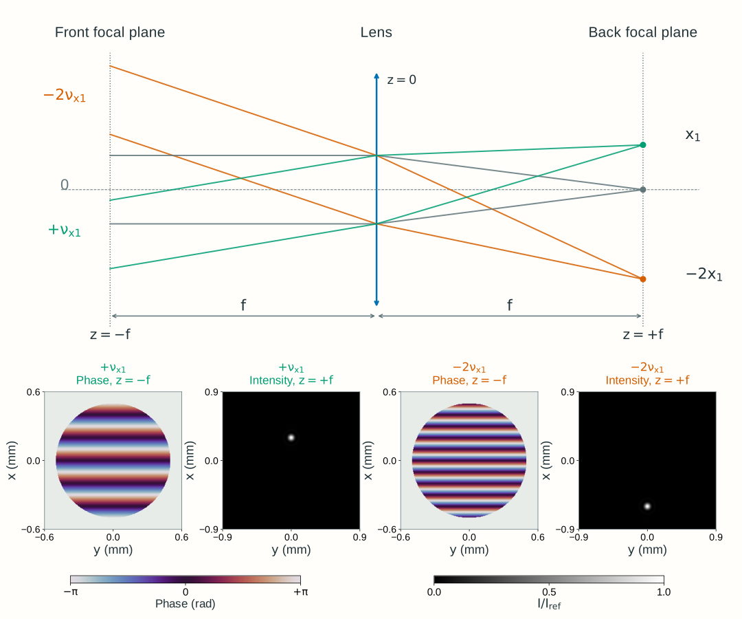
Figure 2.11 illustrates finite illumination: each lower pair uses a disk-windowed tilted field in the front focal plane, with the lens still assumed not to clip the propagated light. The carrier sets the spot center, while the illumination window gives it finite width.
Figure 2.11. A lens separates spatial-frequency components by focal-plane position. Top: two rays per color illustrate one tilt; the geometry is schematic. Bottom: the green and orange fields are calculated separately, each a windowed tilted field with uniform amplitude inside a 1 mm diameter disk in the front focal plane z=-f. The phase maps show this input plane, and the intensity maps show the back focal plane z=+f; the ideal lens introduces no clipping. Phase is wrapped to [-\pi,\pi], with zero phase at the center; the gray region outside the disk is unilluminated. In air, \lambda_0=600~\mathrm{nm}, f=100~\mathrm{mm}, base spatial frequency \nu_{x1}=5~\mathrm{mm^{-1}}, and \nu_{y1}=0 give focal-intensity peaks at (x,y)=(+0.30~\mathrm{mm},0) for the +\nu_{x1} field and (-0.60~\mathrm{mm},0) for the -2\nu_{x1} field. Both intensity maps use the same linear scale, normalized to I_{\mathrm{ref}}, the focal peak for an untilted field with the same illumination. The finite input disk broadens each carrier’s spectrum and produces a finite spot; these windowed fields are not single infinite plane waves. Section 2.4 instead places a finite aperture immediately after the lens and calculates its focal diffraction pattern.
Which input spatial-frequency component corresponds to a given focal-plane position (x,y)? Invert the position mapping:
For an arbitrary input field, evaluate its complex spectrum at these mapped frequencies. Propagating from -f to the ideal lens, applying its quadratic phase, and propagating to +f gives
The spectrum \widetilde U(\nu_x,\nu_y;-f) is the Fourier transform of the input field at z=-f. This is a scaled evaluation of that spectrum, not an identification of position with spatial frequency: x,y have length units, while \nu_x,\nu_y have inverse-length units. The prefactor restores the field scaling and retains the full propagation phase.
The equality holds within the ideal paraxial model, in a common medium, with no lens clipping. Choose the lens’s uniform phase as zero reference, as in Section 2.2. For this front-to-back focal-plane arrangement, the position-dependent quadratic phases cancel. A field specified at the lens plane has different phase bookkeeping; Chapter 2.4 retains the output quadratic phase for that calculation.
Using x,y in both focal planes does not map an input position to the same output position. The back focal plane organizes the input by spatial frequency rather than reproducing its spatial pattern. The second lens introduced below reconstructs an inverted image of that pattern.
A complex pupil changes amplitude and phase
Chapter 1 identified physical apertures and pupils. We now attach a complex transmission to a declared plane z=z_p:
For a passive mask, the real amplitude transmission satisfies 0\le t_p\le1. Its intensity transmission is t_p^2, while \psi_p is the phase added by the element. An opening has transmission one inside and zero outside; a smooth amplitude transmission weights the field gradually; a phase-only plate has t_p=1 and changes phase while preserving local intensity immediately across its plane.
The pupil transmission and the illumination are separate. P describes the element; U(x,y,z_p^-) describes what illuminates it. Their product is the transmitted field. A uniformly open pupil need not contain a uniformly illuminated field.
Placing such a mask in the back focal plane, z_p=f, lets us modify selected spatial-frequency components: an opening controls their amplitudes, while a patterned phase plate changes their phases. The next section adds a second lens to show how these changes affect the reconstructed spatial pattern.
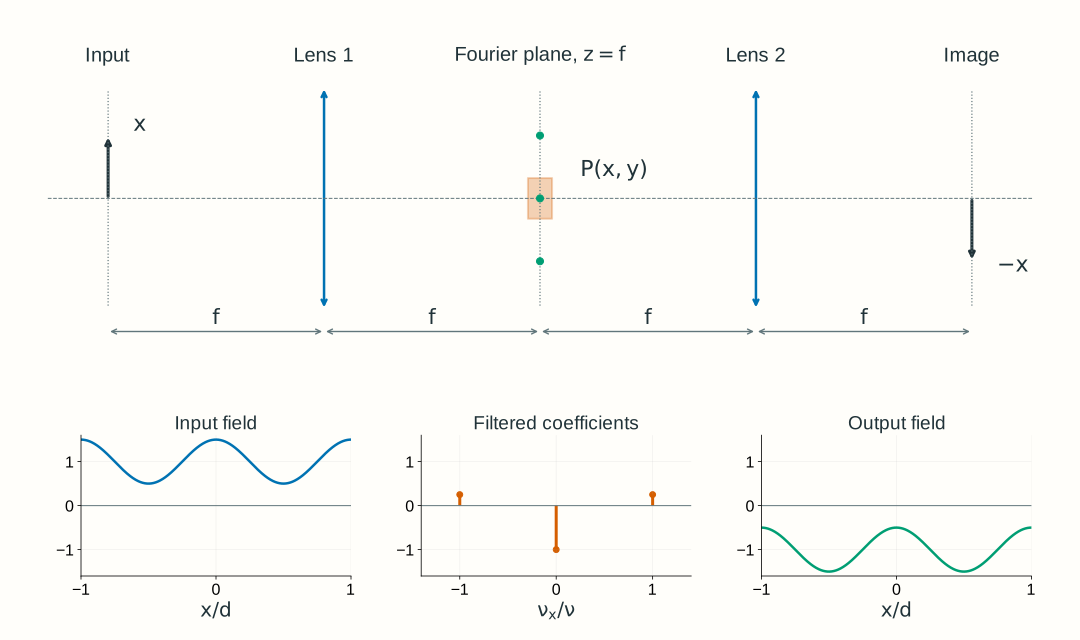
A 4-f relay filters and reconstructs the field
Use two identical converging lenses of focal length f, separated by 2f. With lens 1 at z=0, put the input at z=-f, the common Fourier plane at z=f, lens 2 at z=2f, and the output at z=3f. Every adjacent separation is f. Lens 1 maps input frequencies into positions at the mask; lens 2 recombines the transmitted components into an inverted image.
The relay’s Fourier-plane filter is not automatically its entrance pupil or aperture stop; use Section 1.4’s stop and pupil definitions to identify those planes in a real system.
Figure 2.12. A Fourier-plane mask acts between the decomposition and reconstruction steps. The example changes the central component’s phase by \pi, preserving every component magnitude. The lower field plots omit the common relay factor G=-e^{i4kf}; the negative central coefficient represents a relative phase change. The top arrow marks image inversion. Distances and spectral spots are schematic; the ideal periodic components have zero-width Fourier orders before finite-aperture effects are included.
Write U_{\mathrm{in}}(x,y)=U(x,y,-f) and U_{\mathrm{out}}(x,y)=U(x,y,3f). For a physical mask P(x,y) located at z=f, two successive transforms give
Here G=-e^{i4kf} is the common relay factor. In the spectral integral, P(\lambda f\nu_x,\lambda f\nu_y) means evaluating the physical mask transmission at the position assigned to each input frequency.
Both lenses perform the forward transform in these coordinates. With P=1, two forward transforms produce inversion:
The common factor has unit magnitude and therefore does not change intensity. It matters if this output later interferes with a separate reference field. The equal-focal-length relay has magnification -1; with unequal focal lengths the corresponding ideal magnification is -f_2/f_1.
Blocking an order removes its field contribution. Changing its phase keeps its magnitude but changes how it interferes with the other orders. A phase-only mask can therefore redistribute image intensity without reducing total transmitted power.
Explore: filter and reconstruct a field
Choose all-pass, block-side-orders, or central-order phase reversal, then adjust spatial frequency, the central slit’s half-width, and central-order phase. Compare the input field amplitude, the Fourier components and mask, and the reconstructed output field and intensity. The mask acts on the field coefficients, not on the input intensity.
Model, numerical method, and validation
This is a one-dimensional periodic field, uniform in y, with three exact components: U_{\mathrm{in}}/E_0=1+m\cos(2\pi\nu x). The modulation depth is fixed at m=0.5. It is not a finite beam or a general two-dimensional image. The common medium is air, \lambda=600 nm, and both ideal lenses have f=100 mm. Side orders lie at x=\pm\lambda f\nu; the central order lies at zero. The Fourier-plane slit has half-width a.
The browser evaluates the three complex coefficients and their coherent reconstruction directly on 401 plotted samples over x\in[-0.2,0.2] mm; it does not use an FFT. The plotted field divides out the explicitly declared common relay factor G=-e^{i4kf}, while all intensity curves use I/I_0=|U/E_0|^2, with I_0=\tfrac12n\epsilon_0cE_0^2. This is one fixed normalization, not a separate peak normalization for each curve.
The central phase element acts on the ideal zero-frequency order, with no effect on the other two orders. It represents separated Fourier cells in this discrete model; a finite-width physical phase plate and finite illumination need a continuous-field calculation. Likewise, the slit passes or blocks ideal point orders; it does not simulate finite-pupil diffraction at its edges.
Validation checks all-pass inversion, the wavelength–frequency–position mapping, removal of blocked components, phase-only power conservation over a full spatial period, and the worked-example intensities. Sampling must resolve the selected spatial frequency; refinement changes drawing accuracy, not the analytic three-component model. General FFT workflows additionally require spatial-window, Nyquist, and convergence checks. These teaching choices do not establish Lab 2 software requirements. The standalone explorer retains its complete model explanation.
Worked examples
Guided
Map a spatial period to angle and position
A tilted plane wave in air has vacuum wavelength 600 nm and a transverse phase period d=50~\mu\mathrm m. Its phase increases with positive x. Specify the field at z=-f for an ideal lens at z=0 with f=100 mm. Find its spatial frequency, paraxial angle, and back-focal-plane position.
Hint / setup
Convert all lengths to mm. Use \nu_x=1/d, then \theta_x\approx\lambda\nu_x and x=\lambda f\nu_x. The period refers to field phase, not intensity stripes.
The small positive angle is paraxial and places the component above the axis. Its transverse phase varies, but a single plane wave has uniform intensity. Negative phase slope would give the same displacement magnitude below the axis.
Scaffolded
Remove the side orders
An equal-focal-length 4-f relay in air has f=100 mm and \lambda_0=600 nm. Its input is U_{\mathrm{in}}/E_0=1+0.5\cos(2\pi\nu x) with \nu=10~\mathrm{mm^{-1}}. A centered slit at the common Fourier plane passes |x|\le0.40 mm. Which components pass, and what output field and intensity remain?
Hint / setup
Expand the cosine into its positive and negative exponential terms. Locate all three orders with x=\lambda f\nu_x. Apply the slit to each coefficient and then reconstruct, including or explicitly factoring out G=-e^{i4kf}.
The output is a uniform field with the common relay phase. The input mean intensity over a period was 1+0.5^2/2=9/8 in units of I_0; blocking the two side orders leaves 1. The slit removed field components, rather than directly smoothing an intensity pattern.
Independent
Change phase instead of blocking light
Use the same input and relay as Example 2, with an aperture wide enough to pass all three orders. Compare an unchanged central order, a central-order phase shift of \pi, and a blocked central order. Find output intensity in the plane z=3f at x=0 and x=d/2, where d=1/\nu. Which operation preserves power over a period?
Hint / setup
The central coefficient becomes 1, e^{i\pi}=-1, or 0. The two side coefficients remain 0.25. Reconstruct the field before squaring its magnitude. Inversion does not change this even cosine pattern, and the common relay factor has unit magnitude.
The phase plate swaps the selected bright and dark positions while preserving period-averaged intensity: \langle\cos\rangle=0 and \langle\cos^2\rangle=1/2. Blocking the central order removes its unit contribution to mean intensity. The remaining 0.25\cos^2(2\pi\nu x) has twice the intensity spatial frequency of the cosine field; equal intensities at these two points do not mean a uniform output.
For this ideal periodic field, “power over a period” means the intensity integral over one period per unit extent in y. The infinite field does not have finite total power. The explorer demonstrates the first two cases and blocking the side orders; blocking the central order is the independent extension here.
Model selection and engineering checks
Check what is transformed. Is it the complex field, an intensity pattern, or an intensity PSF? These have different physical meanings. The field spectrum here is not the OTF or MTF from Section 1.6.
Check units. Spatial frequency is in cycles per length; wave-vector components are in radians per length. Use k_x=2\pi\nu_x and medium wavelength in x=\lambda f\nu_x.
Identify the planes. State the input plane, lens planes, Fourier plane, mask plane, and output plane. Reuse stop and pupil definitions rather than calling every aperture a pupil.
Keep the phase conventions. Use a negative exponential for the forward transform and a positive one for the inverse. Retain full propagation phase, or explicitly state a displayed common phase reference.
Check limiting cases. An all-pass equal-f relay returns an inverted field up to the common phase. A phase-only mask preserves component magnitudes and full-field power, although image intensity can change.
Check apertures and paraxiality. Does the real lens transmit the required field without clipping? Are the significant angles small? Ideal separated orders and perfect imaging are limiting models.
Check numerical sampling. For a sampled field, frequencies repeat with period 1/\Delta x and the unique interval extends to |\nu_x|<1/(2\Delta x). A window of width W gives frequency spacing 1/W. Check both window and spacing by refinement before interpreting small features.
Section 2.4 applies the complex pupil to diffraction from a point, then calculates the intensity PSF and its incoherent OTF/MTF. That sequence connects the coherent field calculations here to Chapter 1’s image-contrast requirements.
Further reading
MIT OpenCourseWare, 2.71 Optics: lecture 18 and lecture 19 develop Fourier optics and optical filtering. Compare transform signs, plane definitions, and wavelength conventions before transferring a formula between sources.