Describe the wave that a ray leaves out, add its electric fields, and predict what a detector records.
The engineering question
Two beams overlap on a detector. Will it read the sum of their separate intensities, four times one beam’s intensity, or almost zero? All three outcomes are possible—even when the beams have the same individual intensity. The missing information is how their fields relate during the measurement.
Section 1.6 used a local incoherent-intensity model: responses from object points add in intensity before we evaluate convolution and contrast transfer. We now explain that assumption. The goal is not to repeat the PSF–MTF framework, but to supply the field language needed to extend it to diffraction.
Model
Light as a transverse electromagnetic wave
Begin with a monochromatic plane wave in a homogeneous, isotropic, transparent, nonmagnetic medium. Its electric field \mathbf E and magnetic field \mathbf B oscillate perpendicular to each other and to the propagation direction. Their cross product identifies the energy-flow direction. Polarization describes the electric field’s transverse orientation and motion; for linear polarization, it oscillates along one fixed line.
We will initially track one signed electric-field component, E, along a common linear-polarization axis. This scalar approximation is useful when polarization is fixed and the system does not substantially mix its components. It does not mean the light is unpolarized. Strongly focused fields and polarization-sensitive elements can require a vector treatment. The common-direction assumption also matters when we translate squared field into normal energy flux at a detector.
Electric and magnetic fields in a traveling wave
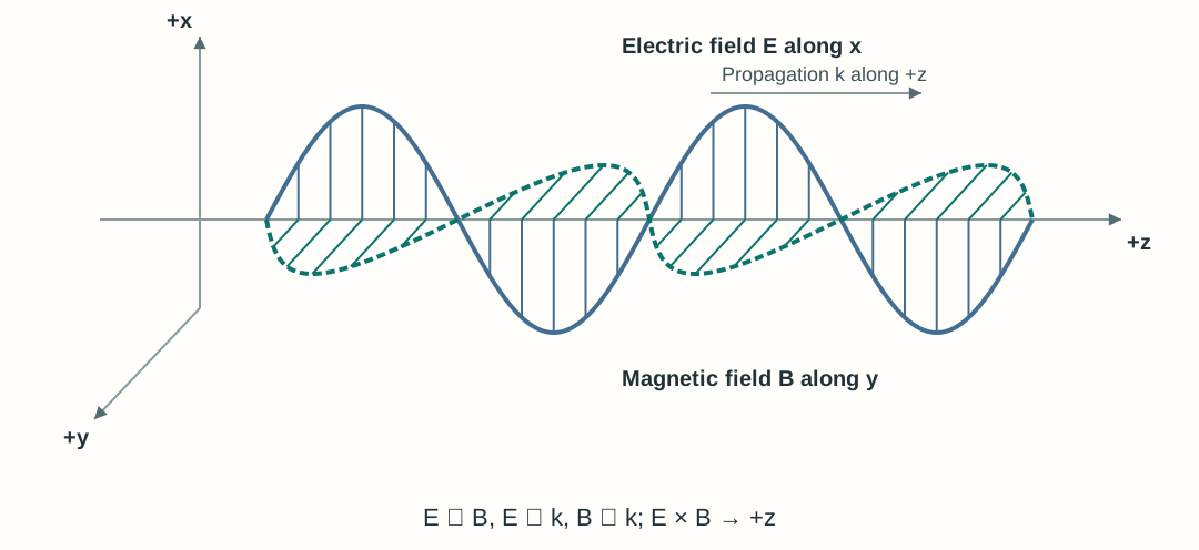
In the classical description, light is an electromagnetic wave: electric and magnetic field values vary across space and in time. Figure 2.1 shows a snapshot of a linearly polarized plane wave traveling along positive z, with \mathbf E along x and \mathbf B along y. At each fixed position, these vectors oscillate along their transverse axes; the curves connect field values at different positions. The field pattern and energy propagate forward. The two field amplitudes use separate schematic scales because electric and magnetic fields have different physical units.
Figure 2.1. Electric and magnetic fields of a linearly polarized plane wave.
A traveling wave carries amplitude and phase
A plane wave has constant phase on planes perpendicular to its wave vector \mathbf k. Its scalar electric field can be written as
The constant E_0\ge0 is the real peak electric-field amplitude, measured in volts per meter (V/m). The constant phase offset \phi_0 is an angle, measured in radians. Angular frequency \omega is measured in radians per second; the magnitude of the wave vector, k=|\mathbf k|, is measured in radians per meter. With ordinary frequency \nu, period T, and wavelength \lambda,
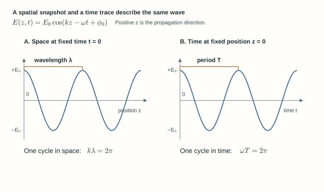
The second relation follows by holding kz-\omega t+\phi_0 constant: the pattern moves toward positive z, consistent with Chapter 1’s coordinate convention. A wavefront is a surface of equal phase. A sinusoidal line plotted along the axis is a field snapshot; it is not a wavefront surface.
Figure 2.2. Space and time offer two views of the same oscillation. The field crosses zero and changes sign; its amplitude is the maximum magnitude. The vertical axis is signed electric field, not intensity and not |E|.
Explore: local oscillation and a traveling pattern
Watch the highlighted observation point (0,0,z_0). Its electric and magnetic field vectors change signed length while their shared origin stays fixed. Neighboring positions have different phases, so the field pattern propagates toward positive z. The wave carries energy; the arrows represent local field values.
Wavelength changes in a medium; frequency does not
Let \lambda_0 denote wavelength in vacuum and n the real refractive index at this frequency. The phase velocity and wavelength in the medium are
Across a stationary, linear dielectric interface, incident, reflected, and transmitted waves have the same temporal frequency. The transmitted wave’s wavelength changes because its phase velocity changes. Its amplitude may also change; knowing wavelength alone does not determine reflected or transmitted power. The velocity here is phase velocity, not a claim about pulse-envelope speed in a dispersive material.
Explore: a wave crosses a glass interface
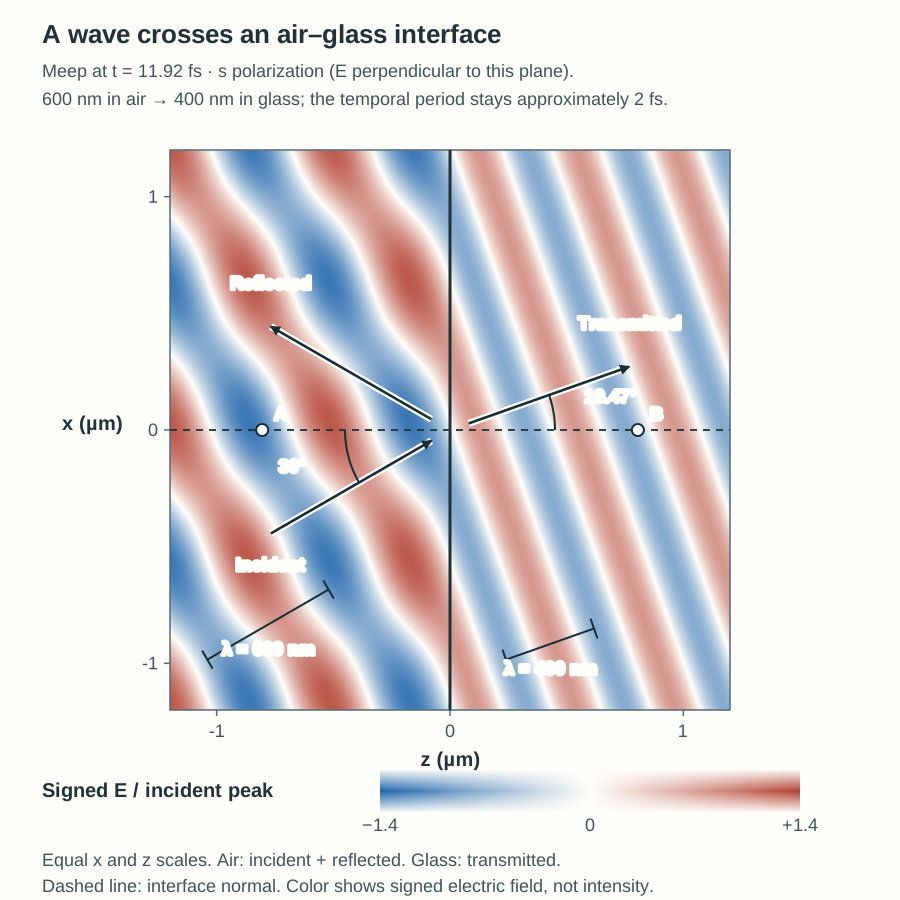
This instructor-prepared Meep model sends a narrowband pulse centered on 600 nm from air with n_1=1.00 into glass with n_2=1.50. The electric field is perpendicular to the drawing plane (s polarization). Measure wavelength along propagation, perpendicular to the wavefronts, and measure angles from the interface normal.
Air–glass interface snapshot. This narrowband Meep snapshot shows the physical total field in air (incident plus reflected) and the transmitted field in glass. Wavelength along propagation changes from approximately 600 nm in air to 400 nm in glass, while the temporal period stays approximately 2 fs. Incidence at 30° gives transmission at approximately 19.5°, measured from the interface normal. Both sides use the same fixed signed-electric-field color scale; the colors do not show intensity.
Start with the incident and transmitted wavefronts; reflection is hidden by default. In the combined view, Show reflected wave adds the reflected component and changes probe A in air from the incident reference to the physical incident-plus-reflected field. Probe B in glass shows the transmitted field. Compare normal and oblique incidence.
Complex amplitude makes phase easier to track
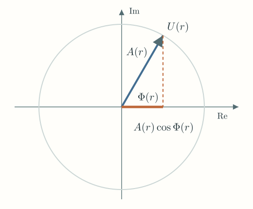
Repeated trigonometric sums become easier if we store amplitude and phase in one complex quantity. Euler’s identity gives e^{i\theta}=\cos\theta+i\sin\theta, with i^2=-1. Define the complex amplitude U(\mathbf r) by
For the monochromatic model, U(\mathbf r) is time-independent: at a fixed position, its magnitude A(\mathbf r) and spatial phase \Phi(\mathbf r) are fixed. The factor e^{-i\omega t} supplies the optical oscillation of the real field.
Here \Phi(\mathbf r) is the full spatial phase, including propagation and the constant offset. For the plane wave above,
The physical field is real. The imaginary part is a mathematical partner that preserves the phase information needed for addition and propagation. The magnitude A(\mathbf r)=|U(\mathbf r)| is the peak field amplitude, and \arg U(\mathbf r)=\Phi(\mathbf r) is its full spatial phase. A complex-plane arrow, or phasor, makes both visible. At one point, multiplying by e^{-i\omega t} rotates that arrow clockwise; its real-axis projection is the instantaneous signed electric field.
Figure 2.3. At a fixed observation point and t=0, the complex-plane arrow has magnitude A(\mathbf r) and phase \Phi(\mathbf r). Its real-axis projection is the signed field E(\mathbf r,0)=A(\mathbf r)\cos\Phi(\mathbf r). This mathematical plane is not a physical transverse plane of the beam.
For the plane wave traveling along positive z, the complex amplitude is U(z)=E_0e^{i(kz+\phi_0)}. Together with our e^{-i\omega t} time convention, this recovers the signed traveling-wave field above. A different time convention is valid if every propagation and phase formula changes consistently.
Two same-frequency waves are added by adding their complex amplitudes. Keep the complex result until after the addition: taking magnitudes too early erases the phase that determines interference.
A detector measures averaged energy flow
An ordinary camera exposure does not follow the sign of the optical electric field on each femtosecond cycle. It responds to energy delivered over an integration interval. For a transverse plane wave incident normally in a lossless nonmagnetic medium, the cycle-averaged energy flux per area is
Here \epsilon_0 is vacuum permittivity, c is vacuum light speed, and |U| is the peak electric-field amplitude, not the root-mean-square (RMS) amplitude. Over one optical cycle, a squared cosine averages to 1/2, so \langle E^2\rangle_{\mathrm{cycle}}=|U|^2/2. This gives the factor of 1/2 in the intensity formula above. For fixed medium and geometry, the essential relationship is I\propto |U|^2. Comparing different media requires retaining the refractive-index factor; arbitrary-angle or vector fields require the relevant normal component of the Poynting vector.
Field amplitude is measured in V/m, intensity in W/m², and total power in W. For normal flux through a detector region D,
P=\int_D I(x,y)\,\mathrm da,\qquad \mathrm da=\mathrm dx\,\mathrm dy
A uniform patch of intensity I covering detector area a has power P=Ia. A detector can therefore collect more power by collecting a larger illuminated area without increasing intensity. In the same medium, doubling field amplitude quadruples intensity. A negative electric-field component indicates direction; intensity remains nonnegative.
Superpose fields before calculating intensity
At one detector location, consider two waves with the same frequency, direction, medium, and linear polarization, with relative phase stable over the exposure. With both spatial phases evaluated at that location, write U_1=A_1e^{i\Phi_1} and U_2=A_2e^{i\Phi_2}. The total complex amplitude is U_1+U_2. Squaring its magnitude gives
For equal component intensities I_0, the result ranges from zero at \Delta\phi=\pi to 4I_0 at zero relative phase. At \pi/2, the reading is 2I_0 even though the phase is stable. Unequal fields cannot cancel completely:
The component intensities are those each field would produce alone at the observation location, after the optical system’s splitting and transmission. A dark region does not destroy optical energy: a complete interference or beam-combiner system redistributes energy among positions or output ports. A local two-field formula alone does not account for every port or source boundary condition.
Explore: two waves and one detector
Adjust relative phase and the second field’s amplitude. The relative phase stays fixed during optical-cycle averaging. The field traces and detector results keep fixed scales so a change in amplitude cannot be hidden by rescaling. The explorer shows static time traces over two optical periods; it does not animate the optical oscillation.
Optical path difference becomes phase difference
For waves derived from a common source, a signed difference in accumulated optical path, \Delta\mathrm{OPL}=\mathrm{OPL}_2-\mathrm{OPL}_1, contributes
The additional term includes initial phase and phase shifts from optical components. An optical-path change of one vacuum wavelength changes phase by 2\pi; half a vacuum wavelength changes it by \pi. Use vacuum wavelength with optical path, or medium wavelength with physical distance in one uniform medium. Do not apply the refractive-index factor twice. Broadband coherence and depth discrimination remain topics for Chapter 3.
When may we add intensities instead?
The fixed-phase result above describes two ideal monochromatic fields. Actual mutually incoherent contributions require a more general description than one pair of fixed, same-frequency phasors: their phase correlation is not maintained under the measurement. The interference cross term then averages to zero, and their measured intensities add:
\overline I=I_1+I_2
Here I_1 and I_2 are the intensities measured from the contributions separately. Optical-cycle averaging alone does not erase a stable relative phase: it is already included in the interference formula. Partial phase correlation can leave a nonzero interference contribution.
Orthogonal polarizations provide a different reason for intensity addition. Their electric-field vectors have zero mutual dot product, so a polarization-insensitive detector has no cross term even if their phases are stable. For general vector amplitudes the relevant term is proportional to \operatorname{Re}(\mathbf U_1\cdot\mathbf U_2^*). A polarizer before detection can project both fields onto one axis and change the outcome. The scalar formula above assumes a common polarization.
Return to Section 1.6’s imaging assumption: when different object contributions are mutually incoherent under the measurement, their intensity responses add, enabling the local intensity-convolution model. Under coherent illumination, the complex field response must be combined first. Linearity and local shift invariance are additional assumptions, not consequences of incoherence. Later sections will distinguish the Fourier transform of a field from the Fourier transform of an intensity PSF.
Explicit temporal phase evolution, broadband coherence, and OCT depth discrimination remain topics for Chapter 3.
Worked examples
Guided
Convert wavelength, intensity, and collected power
A monochromatic wave has vacuum wavelength 600 nm and enters a transparent medium with refractive index 1.50. Find its wavelength, frequency, and period in the medium. In a separate comparison within that same medium, a second plane wave has twice the first wave’s peak electric-field amplitude. What is their intensity ratio? Use c\approx3.00\times10^8~\mathrm{m/s}.
For this separate same-medium comparison, each wave alone uniformly illuminates the same detector area a=2.00~\mathrm{mm^2} at normal incidence. The first wave alone has intensity I_a=10.0~\mathrm{W/m^2}. Calculate the collected powers P_a and P_b from the two waves separately.
Hint / setup
Frequency is set by the source and is unchanged at the stationary interface. First calculate \nu=c/\lambda_0, then use \lambda=\lambda_0/n. The intensity comparison is between two waves in the same medium; square the field-amplitude ratio. Convert square millimeters to square meters before using P=Ia. Evaluate each wave alone; no interference term is needed.
These are powers collected from each wave separately over the same area, not a prediction for two overlapping coherent waves.
The shorter wavelength is consistent with phase velocity c/n=2.00\times10^8~\mathrm{m/s}. Doubling field amplitude gives four times the intensity, not twice. The specified two-wave amplitude comparison does not calculate the interface’s transmission: boundary conditions would be needed for that.
Scaffolded
Interfere unequal beams
Two waves of the same frequency overlap in the same medium, propagation direction, and linear polarization at a detector normal to propagation. Their separate local intensities are I_1=4~\mathrm{W/m^2} and I_2=1~\mathrm{W/m^2}. Write the complex-amplitude ratio U_2/U_1 using \Delta\phi=\Phi_2-\Phi_1. Then predict the detector intensity at stable relative phases zero, \pi/2, and \pi. Can any phase make the detector completely dark? What signed optical-path change moves from zero phase to \pi if the source phases and component phase shifts remain fixed?
Hint / setup
In the same medium, the field-magnitude ratio is the square root of the intensity ratio. Divide the two phasors to retain their relative phase. Then calculate the cross-term coefficient 2\sqrt{I_1I_2} once. Compare field-amplitude magnitudes rather than intensities when considering cancellation. Use vacuum wavelength with optical path.
The three readings are 9, 5, and 1 W/m², respectively. The first field has twice the second field’s magnitude, so opposite phases leave a nonzero field. The minimum is (\sqrt4-\sqrt1)^2=1~\mathrm{W/m^2}. Increasing path 2’s optical path relative to path 1 by \lambda_0/2 produces a phase increase of \pi; any additional integer multiple of \lambda_0 gives the same interference reading. This is a local intensity prediction, not an accounting of every output in a combiner.
Independent
Decide what a reading can establish
Two waves propagate in the same direction in the same medium. Each wave alone gives 2 W/m² at a polarization-insensitive detector normal to propagation. Consider three measurements: (A) common polarization with stable relative phase \pi/2; (B) common polarization with mutually incoherent contributions; (C) orthogonal linear polarizations with stable phase and no analyzer. Predict each reading. Does observing 4 W/m² alone establish that the waves are mutually incoherent? Propose a controlled comparison that separates A from B, with each phase offset held constant throughout its measurement.
Hint / setup
In A, retain the cross term and evaluate it. In B, use the zero averaged interference cross term. In C, consider the vector dot product. Consider repeating measurements at several fixed phase offsets, holding each offset constant throughout its measurement while polarization and component powers remain fixed.
Full solution
All three readings are 4 W/m². In A, the phase is stable but \cos(\pi/2)=0. In B, the averaged interference cross term is zero. In C, the field vectors are orthogonal, so their dot product—and hence the interference term—is zero.
One reading cannot identify which mechanism applies. With common polarization, repeat the measurements at several fixed phase offsets, holding each offset constant throughout its measurement. Case A can give readings from 0 to 8 W/m² across the chosen offsets; case B remains at 4 W/m² while mutual incoherence is maintained under each measurement. Keep individual beam intensities fixed and verify the polarization. Orthogonal polarization can also suppress the fringe, so a flat curve without those controls would not alone establish phase decorrelation. Exposure duration and phase stability are properties of the measurement that must be declared.
Model selection and engineering checks
Which quantity? Is the plot a signed instantaneous field, complex amplitude, intensity, or integrated power? Are its units explicit?
Which wavelength? Use \lambda_0 in vacuum and \lambda_0/n in the medium. Frequency remains unchanged across a stationary linear interface.
Which convention? With e^{-i\omega t}, a forward wave has positive spatial phase e^{ikz}. Use radians in phase calculations.
Which addition rule? Add complex fields before squaring. Add separate intensities only after checking phase correlation, polarization, and detector averaging.
Which normalization? The intensity prefactor assumes peak electric-field amplitudes, common medium, and normal plane-wave flux. A normalized field curve has no absolute W/m² calibration by itself.
Do the limits agree? One zero-amplitude input recovers the other intensity; equal opposite fields cancel locally; unequal fields leave a positive minimum; mutually incoherent contributions recover the intensity sum.
What remains outside scope? This local plane-wave model does not yet predict diffraction, spatial propagation through apertures, polarization mixing, or a complete detector signal with spectral sensitivity and noise.
We can now describe and combine fields at one plane. Section 2.2 will explain how those fields propagate and how a lens changes their phase; the later pupil and diffraction sections will connect that field calculation back to Chapter 1’s PSF, MTF, and contrast requirements.