Connect wavefront curvature to ray direction, then separate a lens’s local phase change from the field formed downstream.
The engineering question
A collimated field reaches a converging lens. Immediately behind the lens, has its intensity already concentrated into a focus? The lens first changes the field’s phase across its aperture. Propagation then combines those phase-shifted contributions into a different spatial field. Keeping these two operations separate explains how focusing works and which approximations support the familiar lens equation.
Section 2.1 supplied the complex amplitude and the rule for adding coherent fields. We now apply them between planes, while retaining Chapter 1’s signed propagation coordinates.
Model
A forward, monochromatic scalar field
Retain Section 2.1’s complex amplitude and full spatial phase:
Here A=|U|\ge0 is real, and \Phi is real wherever the field is nonzero. Monochromatic fixes the temporal dependence at one frequency, making U time-independent. Scalar means that we model one electric-field component under a fixed-polarization approximation. Away from sources and the ideal thin lens, the field propagates in a homogeneous, transparent, nonmagnetic host medium with the same refractive index n on both sides:
This Helmholtz equation follows from substituting the monochromatic time dependence into the scalar wave equation. It does not itself require small propagation angles. Here we additionally select forward fields close to the positive z direction: the paraxial approximation.
The lens lies at z=0; positive x is upward in a meridional drawing. The lens is an ideal phase-only element inside its clear aperture. Reflection, absorption, polarization mixing, and real-lens aberrations are outside this model.
Wavefront normals connect phase to ray direction
A wavefront is a surface of equal phase. Where a smooth local phase and a local propagation direction are meaningful, that direction is parallel to the wavefront normal, given by the phase gradient:
In the meridional x–z plane, the signed angle to the positive z axis follows from the transverse-to-axial ratio of these components. For forward propagation with \partial\Phi/\partial z>0,
For a small angle, the arctangent is approximately its argument. In the local plane-wave interpretation, \partial\Phi/\partial z=k_z\approx k for a forward paraxial field, so
For example, a plane wave traveling in the meridional plane has spatial phase \Phi(x,z)=k_xx+k_zz+\phi_0. Its phase derivatives are \partial\Phi/\partial x=k_x and \partial\Phi/\partial z=k_z, giving
A phase that increases toward positive x tilts the local direction upward. A phase that decreases with x tilts it downward. A constant phase offset changes neither direction nor curvature. The same local relationship applies to the curved wavefronts considered next; it is not a claim that every interfering field, including its zeros, has one unambiguous local ray.
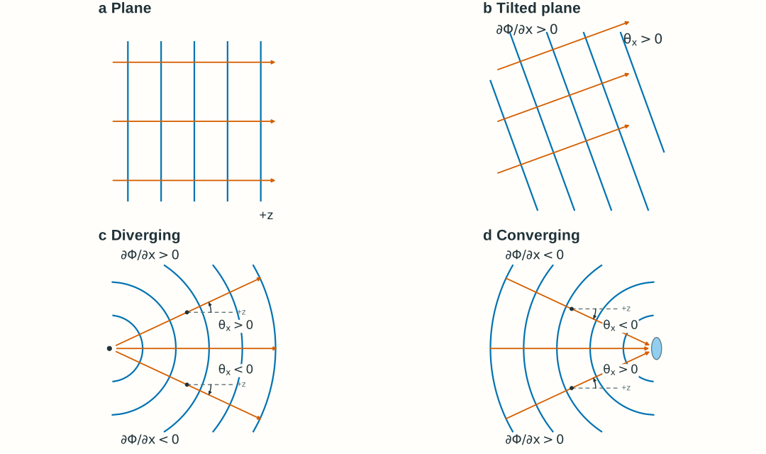
Figure 2.4. Local normals connect phase slope to ray direction. In the diverging and converging panels, the signs of \theta_x and \partial\Phi/\partial x reverse across the axis; both are zero on the axis. The tilted plane has a uniform positive slope and angle. Dashed lines are local references parallel to +z. Wavefront spacing and the relative axial/transverse scales are schematic, not physical measurements; use the phase gradient to calculate direction.
Spherical waves give a quadratic transverse phase
In a homogeneous medium, the scalar wave equation admits spherical-wave solutions as well as the plane-wave solution introduced in Section 2.1. The ideal scalar spherical wave below satisfies the source-free wave equation away from its point source. Its quadratic approximation describes a small region near the axis; the entire spherical wave is not globally paraxial.
Consider an ideal point source on the z axis at (0,0,z_s). Its outgoing spherical wave has the exact spatial form
U(x,y,z)=\frac{C}{s}\exp[i(ks+\phi_0)]
Here s=\sqrt{x^2+y^2+(z-z_s)^2} is the distance from the source. C\ge0 is a real, constant source coefficient with units of field amplitude times length, so C/s is in V/m; \phi_0 is a constant source phase offset. The positive spatial phase matches our e^{-i\omega t} convention.
Choose an observation plane perpendicular to the z axis at coordinate z>z_s. Its axial distance from the source is R=z-z_s>0. If the source is at the origin, R=z. The distance R is constant across this fixed plane and changes when the plane moves along the axis. On the plane, define the transverse radius as r=\sqrt{x^2+y^2}. Then
s=\sqrt{R^2+r^2}\approx R+\frac{r^2}{2R}
For r/R\ll1, approximate the slowly changing amplitude factor by 1/s\approx1/R, while retaining the quadratic change in phase and the full on-axis phase:
The real amplitude and full spatial phase are therefore
A(x,y;R)\approx\frac{C}{R}
\Phi(x,y;R)\approx kR+\frac{kr^2}{2R}+\phi_0
The amplitude is approximately uniform across a small transverse region of a fixed plane. Moving the plane changes R, so its on-axis amplitude falls as 1/R and its on-axis intensity falls as 1/R^2. The quadratic term alone is the transverse phase difference relative to the axis, not the full spatial phase:
\Phi(x,y;R)-\Phi(0,0;R)\approx\frac{kr^2}{2R}
A converging spherical field approaches a point ahead of the plane. Its local form uses e^{-iks}/s, where distance s to that point decreases along propagation. Introduce a signed wavefront radius: R>0 for divergence, R<0 for convergence, and 1/R=0 for a plane wave. Both spherical cases then share the paraxial form
Above the axis, x>0: positive R gives an outward angle, while negative R gives an inward angle toward the axis. See Figure 2.4(c,d) for examples of these local directions.
The radius is signed from the local wavefront geometry; it is not an unsigned object distance. The amplitude A(x,y;R) retains electric-field units. A spherical wave’s amplitude is not exactly uniform over a plane, even when its quadratic phase is a good approximation.
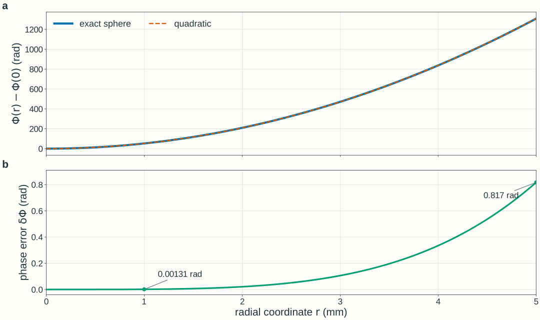
Figure 2.5. Air, R=100~\mathrm{mm}, and \lambda_0=600~\mathrm{nm}. The plotted nonnegative phase error is \delta\Phi=\Phi_{\mathrm{quadratic}}-\Phi_{\mathrm{exact}}, with both phases referenced to the axis. Even a small geometric path error can matter optically. Worked Example 3 compares its magnitude with a stated tolerance.
An ideal thin lens changes phase locally
Write U^- and U^+ for the fields immediately before and after the lens at z=0. An ideal lens of signed focal length f applies
Optional derivation: why does a lens add quadratic phase?
Let a plane wave traveling along +z reach a converging lens at z=0, with the intended focus at (0,0,f), where f>0. Define r^2=x^2+y^2. The distance from a point (x,y,0) in the lens plane to the focus is s=\sqrt{f^2+r^2}.
The off-axis propagation path is longer than the on-axis path. To make contributions arrive at the focus with matching phase, the lens compensates this extra propagation phase. A refractive lens supplies the phase difference through its varying optical thickness:
The quadratic approximation requires r/f\ll1. Choosing the uniform center phase as the reference then gives the lens transfer above. This argument uses phase matching and the paraxial path expansion; it does not assume the ray thin-lens imaging equation, which the main text recovers below.
We choose the lens transmission phase at its center as the reference, omitting a spatially uniform lens phase delay. This convention removes only that uniform delay, not the input field’s on-axis phase. Inside the clear aperture, this multiplier has unit magnitude, so |U^+|^2=|U^-|^2. The intensity does not suddenly concentrate at the lens plane. An aperture that clips the field is an additional amplitude operation and can remove power.
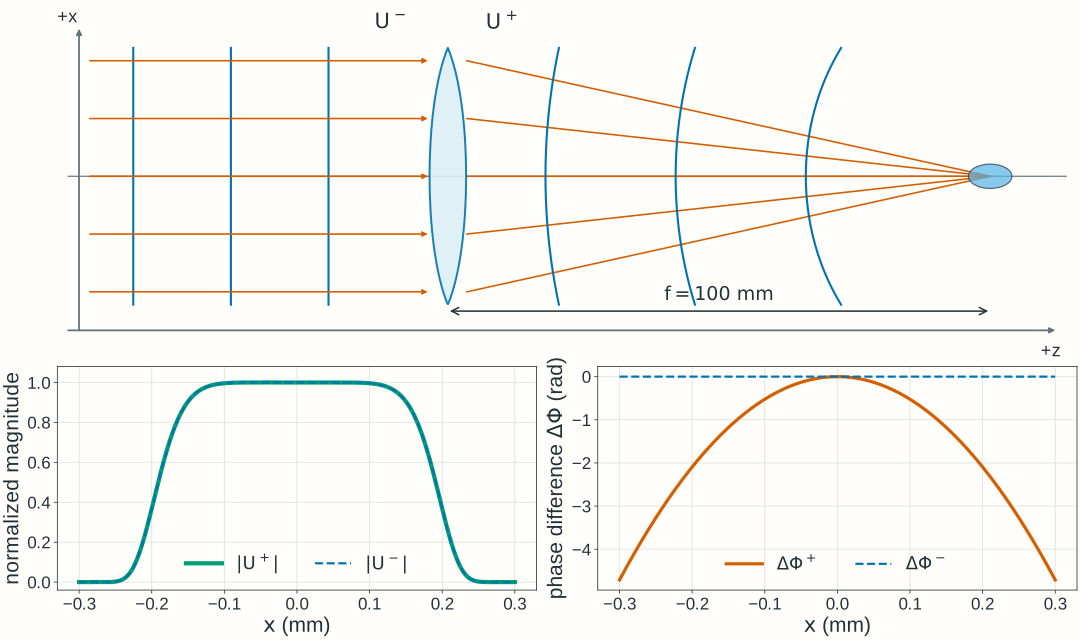
For the converging lens illustrated in Figure 2.6, an incident field with planar wavefronts acquires the negative quadratic phase -kr^2/(2f). This matches the paraxial phase of spherical wavefronts converging toward (0,0,f). The field magnitude remains unchanged immediately across the lens; subsequent propagation brings the contributions together into a finite focal spot. The focal region in the figure is schematic.
Figure 2.6. A lens changes phase at one plane; propagation changes the spatial field between planes. The magnitude curves use an assumed finite illumination profile for illustration; the ideal phase-only lens preserves this profile immediately across its plane. The lower phase curves show differences relative to the axis, \Delta\Phi^\pm(x)=\Phi^\pm(x,0)-\Phi^\pm(0,0). Axial/transverse scales and wavefront spacing are schematic. The finite focal region is shown qualitatively, not as a computed PSF.
From lens phase to the thin-lens equation
Now consider an incident field with spherical wavefronts of signed radius R_{\mathrm{in}} at the lens plane. Its paraxial form is
Here A^-=|U^-|\ge0 is the real field amplitude and \Phi^-(0,0) is its on-axis phase. Spherical wavefronts specify the phase geometry; A^-(x,y) allows a general illumination profile, including a uniform one. For the near-axis point-source approximation introduced above, the amplitude is approximately uniform across a small illuminated region of the lens plane. Its profile does not enter the following phase-curvature calculation because the ideal phase-only lens preserves it. Adding the incident transverse phase difference to the lens’s quadratic phase gives:
The output phase has the same quadratic form as the paraxial phase of a spherical wave. We can therefore describe its wavefronts within this approximation by a new signed radius R_{\mathrm{out}}, with a plane wavefront as the zero-curvature limit. Matching the phase curvature does not imply that the output amplitude has the form of an exact spherical-wave solution.
Matching this quadratic coefficient to the output spherical-wave phase gives the curvature rule:
A plane input has 1/R_{\mathrm{in}}=0, so a converging lens produces R_{\mathrm{out}}=-f. The phase-gradient relation also gives \theta_{x,\mathrm{out}}=\theta_{x,\mathrm{in}}-x/f, matching the thin-lens ray-angle change from Chapter 1.
For a spherical field from an axial object, R_{\mathrm{in}}=-z_{\mathrm{o}}. A paraxial real image at z_{\mathrm{i}}>0 corresponds to R_{\mathrm{out}}=-z_{\mathrm{i}}. Thus the curvature rule recovers the signed imaging relation:
This predicts a geometric conjugate or collimation condition. A finite illuminated field propagates to a finite wave pattern rather than an infinite-intensity point. Sections 2.3–2.4 develop the Fourier and diffraction-PSF descriptions; Gaussian-beam parameters are introduced in Section 2.6.
Paraxial propagation combines fields from a plane
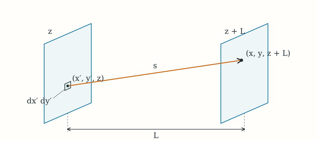
How does a known complex field at one transverse plane determine the field downstream in a homogeneous medium? Consider an input plane at z and an observation plane at z+L, separated by L>0.
Figure 2.7. Fresnel-kernel geometry. A small input patch at (x\prime,y\prime,z) contributes to the field at (x,y,z+L) along a path of length s; L is the axial separation between the planes. The geometry and patch area are schematic, not to scale.
The distance from a small input patch at (x',y',z) to the observation point (x,y,z+L) is
s=\sqrt{L^2+(x-x')^2+(y-y')^2}
In the scalar diffraction model, each patch acts as a mathematical secondary source. Its local complex field supplies amplitude and phase; a complex propagation weight, the kernel K_L, gives its contribution to the observation point:
In the small-angle scalar diffraction model, the propagation weight is approximately
K_L(x-x',y-y')\approx\frac{1}{i\lambda L}e^{iks}
Here s is the geometric path length. Scalar diffraction theory supplies the normalization; the prefactor already uses the near-axis approximation for the propagation weighting. We next approximate the path length in the phase.
For small transverse separations compared with L, use the same paraxial path expansion introduced for the spherical wave:
s\approx L+\frac{(x-x')^2+(y-y')^2}{2L}
The propagation phase ks then separates into an axial part and an additional part from transverse separation:
Here \lambda=\lambda_0/n is the wavelength in the propagation medium, and k=2\pi/\lambda. The kernel has units of inverse area, so multiplying by the patch area leaves field units. Summing the contributions from the entire input plane gives the Fresnel integral:
The integral adds complex field contributions: matching phases reinforce, while differing phases can partly or fully cancel. Calculate intensity only after the sum. This is not Chapter 1’s incoherent intensity-PSF convolution. At L=0, use the input field directly rather than the integral’s singular-looking prefactor.
The paraxial path approximation must give adequate accumulated phase accuracy over the contributing region, propagation distance, and aperture required by the task. Small angles alone do not guarantee that phase accuracy. Section 2.3 describes the same propagation through spatial-frequency components.
For the lens example, take U(x,y,0)=U^+(x,y), the field immediately after the lens. Propagate downstream to U(x,y,L) to determine how its changed phase produces the intensity distribution.
Explore: lens phase and downstream intensity
Choose plane-to-focus, diverging-to-collimated, or finite-image illumination, then adjust input vergence V_{\mathrm{in}}=1/R_{\mathrm{in}}, focal length, and observation distance. Positive input vergence here means a diverging wavefront because R_{\mathrm{in}}>0. Compare the meridional wavefront schematic, lens-plane phase, and calculated central intensity profile. Each setting describes a stationary monochromatic field; there are no animation or pulse-propagation controls.
Model, numerical method, and validation
The explorer propagates a two-dimensional scalar field with a fixed, smooth circular illumination profile,
A(r)=E_0\exp[-(r/w)^8],\qquad w=0.80~\mathrm{mm}
Here E_0 is the input peak electric-field amplitude in V/m; the numerical field may be normalized by E_0. The parameter w is a scale radius, not a Gaussian-beam waist. The profile limits the illuminated region smoothly, with scale diameter 1.60 mm and no hard edge. The larger illuminated region keeps the wave-intensity maximum close to the geometric axis crossing; finite-aperture diffraction can still produce a small shift. The intensity display uses the same input-peak normalization and fixed scale across settings, rather than renormalizing every curve to its own peak. The meridional picture is a schematic of curvature, not a calculation of a full three-dimensional field or intensity along a ray.
The input on-axis phase and the lens’s uniform phase delay are chosen as zero reference values. The lens multiplies the field by \exp[-ikr^2/(2f)]. The finite field continues to spread even when its phase immediately after the lens is planar.
Propagation uses a 1024 × 1024 square field on x,y ∈ [−3, 3) mm (5.859375 µm spacing). The paraxial transfer factor is exp(ikL) exp[−iL(kₓ² + kᵧ²)/(2k)]. Returned complex samples represent the full U/E₀, including the common axial phase exp(ikL); that common phase does not change intensity. For plotting, the complex central field is Fourier-interpolated to 1.464844 µm spacing before taking its squared magnitude; this does not add physical resolution to the two-dimensional simulation. The full two-dimensional power integral is conserved by this phase-only propagation in a common medium.
Checks compare zero-distance identity, curvature signs, integrated power, and central profiles after grid and window refinement. At the selected boundary/reference cases, doubling the sample count changes the central complex field and intensity by less than 10⁻⁸ of input peak field and intensity, respectively; doubling the window at fixed spacing changes them by less than 10⁻⁶ and 10⁻⁶, respectively. Independent radial Fresnel integrals also check the narrow focal profiles and axial peak positions. The finite FFT window is periodic; these checks apply to the stated controls, illumination, and viewing region.
The reference calculations use NumPy/SciPy; the browser evaluates the same scalar model in JavaScript. Check spatial sampling, numerical window, and refinement before interpreting a computed peak. These numerical teaching choices do not set Lab 2 software requirements.
Worked examples
Guided
Find lens phase and local deflection
A plane wave of vacuum wavelength 600 nm reaches an ideal converging lens in air. The focal length is f=100~\mathrm{mm}. At the selected illuminated edge x=0.20~\mathrm{mm}, y=0, find the lens phase relative to its center and the outgoing local angle. Does the phase-only lens change intensity immediately across its plane?
Hint / setup
Use wavelength in millimeters with the other lengths. Evaluate \Delta\Phi_{\mathrm{lens}}=-kx^2/(2f). Differentiate the lens phase for the angle, or use \theta_{x,\mathrm{out}}=-x/f for a plane input.
The reported lens phase is relative to the lens center; the full input field need not have zero on-axis phase. At positive x, the negative angle points toward the axis. The angles are small, consistent with the paraxial model. Inside the clear aperture, intensity is unchanged immediately across the ideal lens; the downstream distribution changes through propagation.
Scaffolded
Connect curvature to the signed image location
A diverging spherical field reaches a thin lens with R_{\mathrm{in}}=150~\mathrm{mm}. The lens has f=100~\mathrm{mm} in the same host medium on both sides. Predict the output curvature and paraxial image coordinate. Translate the input curvature into the signed object coordinate and check the result with Chapter 1’s lens equation.
Hint / setup
Subtract lens power from input curvature. A negative output radius means convergence, while a positive real image coordinate lies downstream. Use z_{\mathrm{o}}=-R_{\mathrm{in}} and z_{\mathrm{i}}=-R_{\mathrm{out}}.
The field leaving the lens is converging. The coordinate 300 mm is its paraxial conjugate prediction, not a claim that a finite illuminated field makes an infinitely bright point there.
Independent
Check whether a quadratic phase is accurate enough
An exactly spherical diverging wave in air has radius R=100~\mathrm{mm} at an ideal quadratic-phase lens with f=100~\mathrm{mm}. Its vacuum wavelength is 600 nm. Predict collimation from curvature, then test that approximation over illuminated radii 1.00 mm and 5.00 mm. The task requires residual phase magnitude no greater than 0.10 rad relative to the on-axis phase. Which radius satisfies that requirement? This is a phase-approximation check, not a real-lens aberration calculation.
Hint / setup
At y=0, evaluate the exact spherical phase and its quadratic paraxial approximation at x=1.00~\mathrm{mm} and x=5.00~\mathrm{mm}, with both phases referenced to the axis. The lens subtracts the quadratic phase, so the remaining phase is the exact-minus-paraxial difference. Compare its magnitude with 0.10 rad.
Use lengths in millimeters and k=2\pi/0.000600~\mathrm{mm^{-1}}. Evaluate with full calculator precision before subtracting; the table values are rounded. These are unwrapped phase differences, not phases reduced modulo 2\pi.
x (mm)
Exact (rad)
Paraxial (rad)
Difference magnitude (rad)
1.00
52.358569
52.359878
0.001309
5.00
1308.179837
1308.996939
0.817102
The lens subtracts the paraxial quadratic phase because f=R. The difference magnitude in the last column is therefore the residual phase magnitude after the lens, relative to the axis. The 1 mm radius passes the 0.10 rad requirement; the 5 mm radius fails. Both have small geometric ratios, 0.01 and 0.05, but the larger patch has too much phase error for this requirement. Matching curvature cancels the quadratic term; it does not make the exact spherical input perfectly planar over an arbitrary radius or establish uniform amplitude.
Model selection and engineering checks
Separate the operations. Did you apply the local lens phase before propagating the field to a different plane? Does the intensity remain unchanged immediately across an unclipped ideal phase-only lens?
Check signs. Positive R means divergence; negative R means convergence. Convert R_{\mathrm{in}}=-z_{\mathrm{o}} and R_{\mathrm{out}}=-z_{\mathrm{i}} before using the signed lens equation.
Check units and conventions. Use medium wavelength with k=2\pi n/\lambda_0, consistent length units, radians for phase, and e^{-i\omega t} with forward e^{ikz}.
Test the approximation against the task. Are the significant propagation angles small, and is the accumulated phase error acceptable over the full illuminated region and propagation distance?
Add coherent fields. Compute intensity after propagation and field addition. A meridional wavefront sketch does not determine the full two-dimensional intensity pattern.
Check numerical sampling. Resolve transverse amplitude and phase, include a sufficiently large spatial window, and repeat with a refined grid and window. A fixed display scale makes comparisons readable; it does not establish convergence.
Check power. An unclipped phase-only lens preserves field magnitude and power. Ideal Fresnel propagation conserves the full-plane integral of intensity within this scalar model; a finite observation window may miss redistributed power.
Section 2.3 will connect these plane-to-plane field relationships to spatial frequencies and the complex pupil. Quantitative diffraction PSFs and MTF follow in Section 2.4; Gaussian-beam transformations follow later in Chapter 2.
Further reading
MIT OpenCourseWare, 2.71 Optics: wave-optics lecture notes develop propagation from an aperture and the quadratic phase of a thin lens. The notation here retains our medium wavelength and signed axial convention; Fourier-plane interpretations are developed in Section 2.3.